Introduction
The Equinox Marathon is one of the more difficult marathons in the world, with over 3,000 feet of elevation gain (and loss), often difficult weather conditions, and a mixture of trail and road. It was started in 1963 and has been run every year except 1992 when heavy snowfall made the course too difficult to support and this year when the COVID-19 pandemic made it unsafe for racers and supporters to gather. In both 1992 and this year participants raced the course unofficially. I was one of the unoffical participants in 2020, my fourth running of the marathon.
Preparation
Because of the pandemic, I haven’t been bicycling to work every day (or much at all), and I picked up the slack by running. Except for the weeks surrounding my backpacking trip to the White Clouds Wilderness in July, my weekly mileage has been above 20 miles since March, and above 30 miles per week since May. While that’s a great base, my longest run prior to the marathon was only 16 miles, and the majority of other long runs I did were between 10‒13 miles. I also tapered for only one week. Since this wasn’t an official race and I was underprepared, I decided to try to take it easy and avoid some of the issues I’ve had in past years with cramping, knee pain, and in 2013 when I damaged the labrum in my right hip.
Race Start
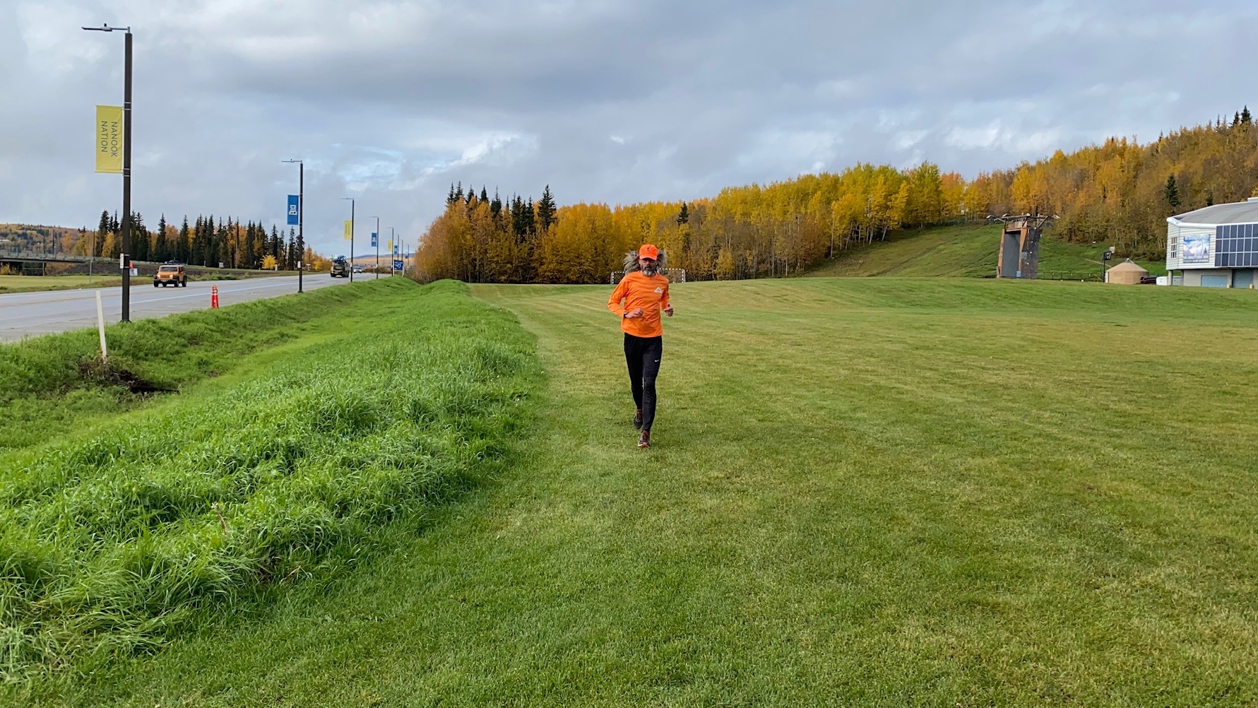
We got to UAF a few minutes before eight. Andrea supported me for the whole race, meeting me at the muskox farm, Yankovich and Miller Hill, Ann’s Greenhouses, at the top of Ester Dome, the mine at mile 20, at the end of the power line, and near the Sheep Creek pullout on campus. I didn’t need much except refills of my water, but it was lonely out there without all the other racers, water stops, and all the community that typically comes out for Equinox.
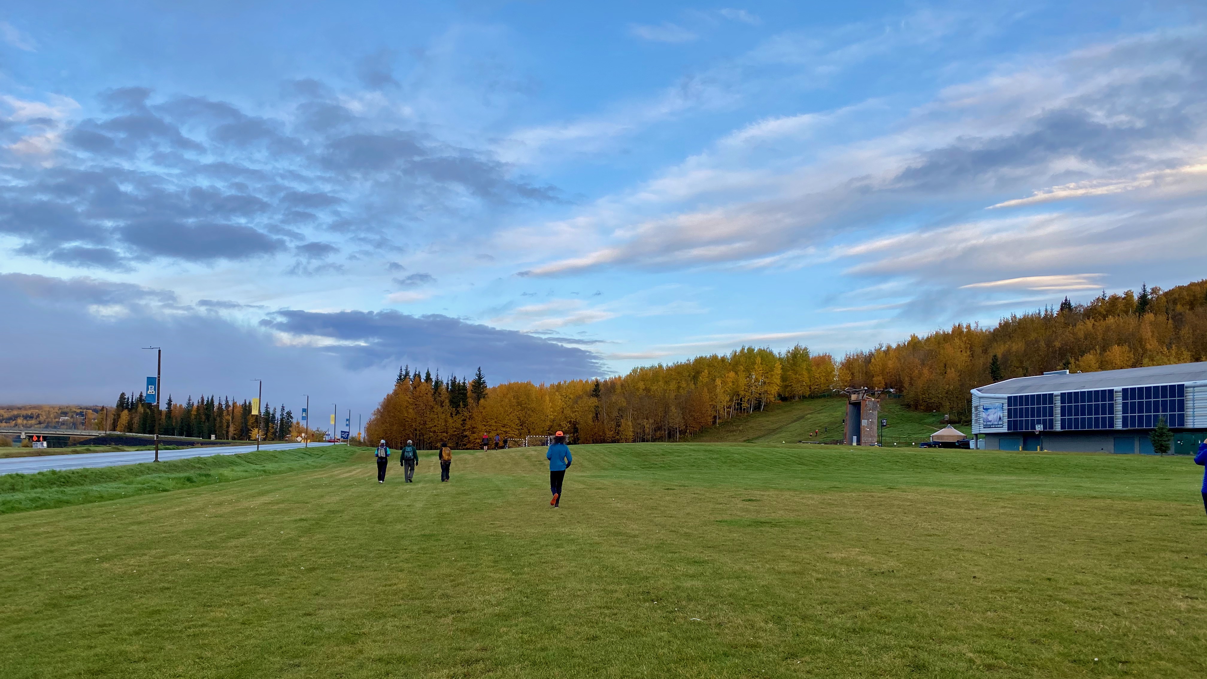
Equinox Marathon start
It was in the mid-30s, cloudy, and humid since it had rained overnight. The grass was wet. About 30 people came to run or hike the course, most starting at 8, but some later. Thick clouds completely obscured Ester Dome which would ordinarily have been visible on the drove over to UAF. Race director Stacy Fisk announced the start, but I held back for a minute to let the pack get ahead of me.
I wore Brooks Cascadia shoes, calf-high thick wool socks, running pants, long sleeve technical shirt (the orange 2017 Equinox Marathon race shirt), Patagonia Airshed pullover, lightweight gloves, and my bright-orange ABR field hat.
First five miles
The first five miles start at UAF, go straight up the sledding hill to the left of Patty Center and around the trees to a sidewalk that goes from the UAF Museum, past the Natural Sciences Building, to the campus dorms where the trail turns left and heads down the hill to the Skarland ski trails.
I jogged a bit to the sledding hill, but walked most of the way to the sidewalk, where I started running for real. It felt good, and I stretched it out a bit running down the hill to the trails. I’ve run the Skarland Loop on campus multiple times each week all summer, so hitting the “A” entrance, I felt like I was on my home trails. Running downhill toward Ballaine Lake, you could feel the temperature drop. The leaves on the trees and shrubs next to the trail were crispy with frost.
The trail parallels Ballaine Road until it runs into Ballaine Lake where there’s a brief diversion onto the bike path and back onto trails before the campus outdoor shooting range. Back into the woods I caught Bob and Sharon Baker just before mile two sign with their names on it.
Just after mile two the trail goes out onto Ballaine Road briefly, dips back into the woods for a half mile or so, then comes back out onto the road. Personally, I hate these particular road sections because you are running uphill on the pavement and there’s a lot of very fast moving traffic coming right at you down Ballaine Hill. It started raining.
The trail section between mile three and five after getting off Ballaine Road were really pretty, despite the light rain. It’s mostly mature birch forest with little ground cover and the bright white and black tree trunks with a forest floor covered in yellow leaves was exceptional. There’s some hills in this stretch as well, gaining and losing around three hundred feet. I walked some of the steeper hills and loped back down them.
The house at the corner of Dalton and Sandpiper, which is the high point of this section of the trail had a big sign pointing toward their outhouse. You can’t miss the house because it’s got a giant solar array on a post, and a second array on a nearby shed. I didn’t need the outhouse, but it being there was appreciated. As I crossed Sandpiper, the owner (local politician and Ph.D. geophysicist John Davies) wished me a good run and I thanked him for the outhouse.
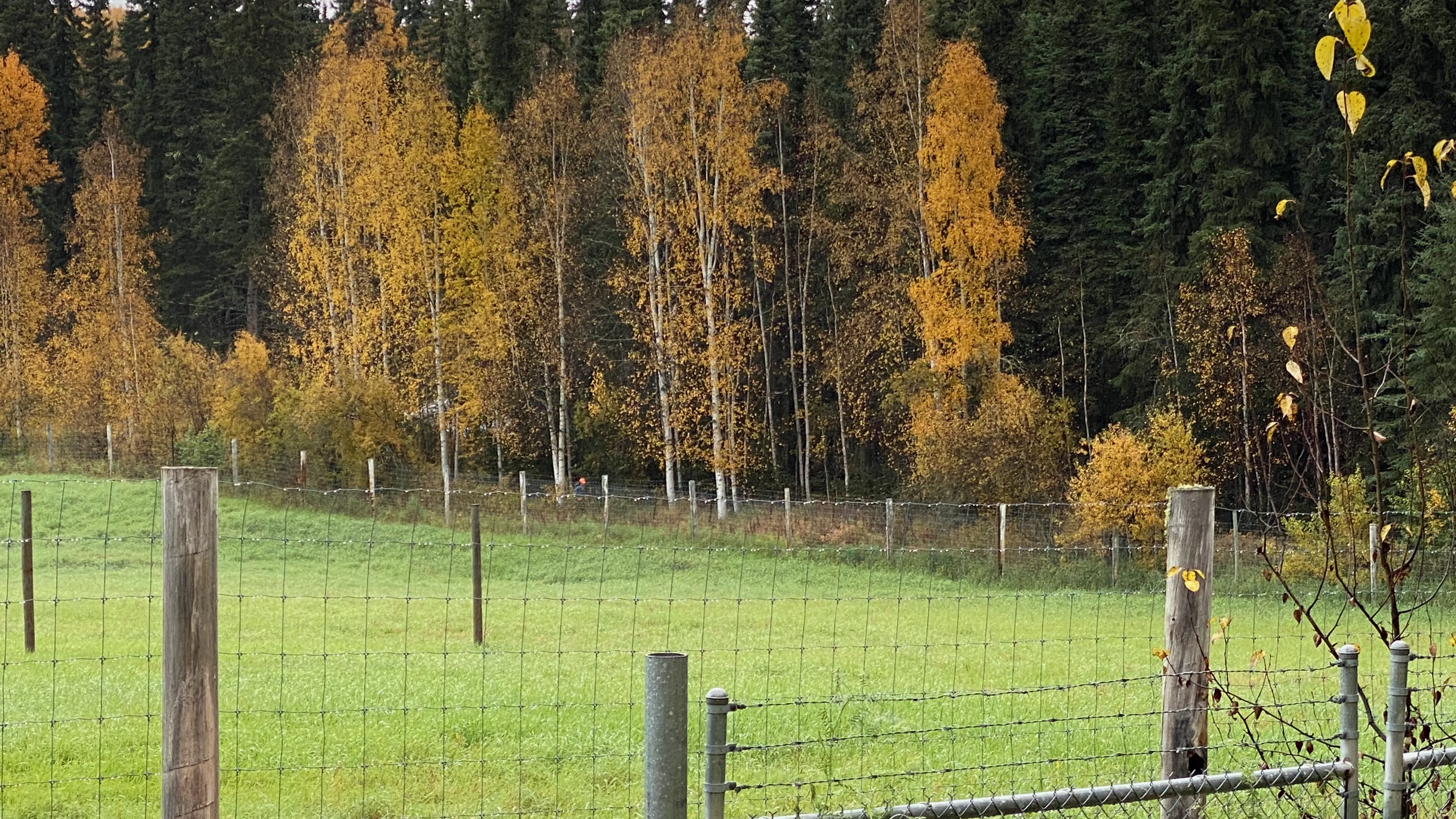
Along the fence at the muskox farm
At the muskox farm the trail crosses Yankovich Road and follows more of the Skarland trail on UAF’s north campus. More of that home trail feeling. Running up past the mile five sign I remembered being stalked by a Northern Goshawk on an early spring run many years ago.
To Ester Dome
After running up to the top of Miller Hill on the UAF trails, there is another road crossing at the intersection of Miller Hill and Yankovich Road, just up the hill from our house. This is a good spot to watch the early leaders in the race and there's normally a water stop at this intersection. Next, the trail follows a power line easement along Lawlor, oriented directly at Ester Dome, so you can typically see exactly what you will be running up starting in another four miles. Not this year. Rain was still falling, and Ester Dome was completely obscured by low clouds.
Crossing Miller Hill and Yankovich
The course comes off the power line easement onto Lawlor Road, past Moving Free Farm, and down a steep dirt road that eventually leads back onto a rutted trail running through deep boreal forest. In the winter, I often run the commuter trail that goes through our property and after a mile head up the hill to this trail, which leads to the edge of the hay field on Sheep Creek. Coming out at the top of the hay fields into the sun in the middle of winter is pretty great.
The trail comes out on a couple gravel roads. In a normal year there is a crowd of people cheering on runners, but this year it was quiet. I passed a couple people walking down Line Drive, down Black Sheep and onto the path next to Sheep Creek. The first year Andrea did Team In Training she ran the last leg of the relay and her sister ran the first leg. That was a bad yellow jacket year and whenever I’m running on this stretch of the trail I remember her shouting to us, “I just got stung by a bee!” as we drove to meet her at the first relay exchange (she was fine).
At the railroad tracks the Equinox Trail crosses Sheep Creek and runners head across the railroad tracks and through the fields on the other side of the street from Ann’s Greenhouses. This section is private property, so I ran on the road toward Goldstream Sports and Ester Dome Road. Andrea met me there and refilled my water bottle with more water and Tailwind.
There’s about a mile of road between Ann’s Greenhouses and where the single track starts winding up Ester Dome. Much of my training this spring and summer involved parking at the pullout past Ann’s, running up Ester Dome on the course, then back down via Henderson or St. Pats to the truck. So this section felt very familiar, except this time I had already run more than eight miles getting there.
Up the Dome
The single track winds around and up through a mature birch forest until hitting Ester Dome Road 285 feet higher in elevation. The trail crosses the road, re-enters the woods, follows the hillside contour for a short distance, then turns directly uphill at the mile 10 sign. I ate a packet of Honey Stingers as I trudged up the hill.
Up and up, past a derelict car that must have a thousand bullet holes in it and through mile 11 where it finally levels out for a quarter mile before intersecting Ester Dome road for the second time near the intersection with Henderson Road. There’s a short side trail off on the left where the trail levels out where people (OK, me!) often duck in to go to the bathroom. I’d already stopped along the trail between Lawlor and Black Sheep, so I didn’t need it this time. Now we are 900 feet from where the single track started, and 1,180 feet higher than the start at Patty Center.
The rain picked up on the single track, but by the time I made it back to Ester Dome Road past mile 11 we were deep inside the clouds that were raining on Fairbanks below, and it was more like a damp fog than actual rain. I walked up most of the steeper sections, and walked up the first part of Ester Dome Road past Henderson.
Just before the mile 12 marker, the road curves to the right and there’s a panoramic view of Fairbanks, the Tanana River, and the Alaska Range behind it. On this day, you couldn’t see more than a hundred feet into the clouds, so it felt like looking off the edge of the world. In last year’s race it was snowing and the wind was howling in our faces at this stage, and I remember looking down and watching the snow collect in the hair on my legs, pulling my wind shirt tight to keep the hood from blowing off.
There are a few houses along the road here, and on my previous runs I often encountered a loose dog whose owner would shout from behind the trees, “That’s Kimber, she’s friendly,” and then “See you on the 19th.” On my last run up Ester Dome two weeks before the race I asked him if he realized the race was cancelled and he said, “I’ll be up here. Will you?”
Sure enough, as I got closer, I could see a figure in the road through the fog; eventually three people, a table and some cups filled with beer. He was dressed in jeans, boots, and a sport coat, offered me a beer, and had his companions start playing their guitars for me. Such a strange scene. Temperatures in the mid-30s, shrouded in clouds, one tired runner (me), one extremely animated man shouting about running and politics, and two guys playing guitar and bass while I drank my beer up near the top of Ester Dome. I spent a few minutes hanging out with them before continuing on.
Up on top of Ester Dome
New trails
The course at the top of Ester Dome has changed many times over the years because some of the property at the top is private property, owned by the Alaska Ski Corporation, and they have been militantly protective of their private property rights. They only grant access to cross their parcels on race day, and in past years have waited until just before the race to allow or deny access to trails people have been running on for decades. Not only does that make it difficult to set a course when it might need to be drastically altered at the last minute, but it means that people aren’t allowed to train on the race course without trespassing. The “Goat Track,” “Zipper,” and “Alder Chute” are all sections of the trail memorable enough to get names, but are accessible only by the whims of the Alaska Ski Corporation.
The Interior Trails Preservation Coalition (ITPC) has been pursuing alternative routes for this section for years, and finally got legal authorization from the Alaska Department of Natural Resources (DNR) to cut trails along the section line easement that crosses Alaska Ski Corporation land. This new route is not officially part of the Equinox Marathon course, but since this year’s race was unofficial and we didn’t have the Alaska Ski Corporation’s permission to run on the Zipper and Alder Chute, these new trails were our only alternative if we wanted to run Equinox without trespassing. The Alaska Ski Corporation disputes the DNR ruling, but unless they get a court to overrule DNR, these section line trails are legally accessible to runner.
There was a rumor that the Alaska Ski Corporation agent would be out on the course threatening runners who attempted to use the new trails, but no one confronted me, and there were no additional signs or warnings, so after running through the Tunnel, and along Ester Dome Road to the entrance of Styx River Road, I turned north along the new section line trail leading up past the first set of towers. Andrea met me just before entering the new trail and offered me a carrot from Spinach Creek Farms that she’d gotten at the Farmer’s Market while I was climbing Ester dome. I ate it on my way up to the towers at the top of Ester Dome.
The new trail is awesome, running mostly straight through open boreal/alpine forest. The mosses and lichens covering the ground were fully expanded and bright, and the leaves on the low shrubs had all turned bright yellow, orange, and deeply red for autumn. Up the hillside to the left, the towers and other buildings faded in and out through the fog.
The trail eventually intersects an old four wheeler track just past last year’s mile 13 marker which takes you up to the first set of towers, then back down to Ester Dome Road. This is the high point of the course; by my watch, elevation 2,385 feet.
Two years ago, coming down this little hill from the towers toward the second relay exchange, both of my hamstrings locked up and I had to stop and stretch them out. The cramps in my hamstrings stuck with me for the rest of the race, making for a very challenging and slow finish because I had to keep stopping to stretch them out every few minutes. I leap-frogged most of the last six miles of the race with another guy who’s quads were cramping and we must have looked strange, me bending over to stretch my hamstrings, him squatting deeply to stretch his quads.
This time I could feel that my right hamstring was tight, and maybe a little tired, but under control. A small collection of vehicles had gathered by the fire service water tank at the second relay exchange, including our truck, and the people there cheered as I ran past. Andrea had thought I was going to run up the road instead of taking the new trail so I saw here coming back up the road and I yelled to her that I’d taken the “illegal” trail. Some of the people laughed.
Out and Back
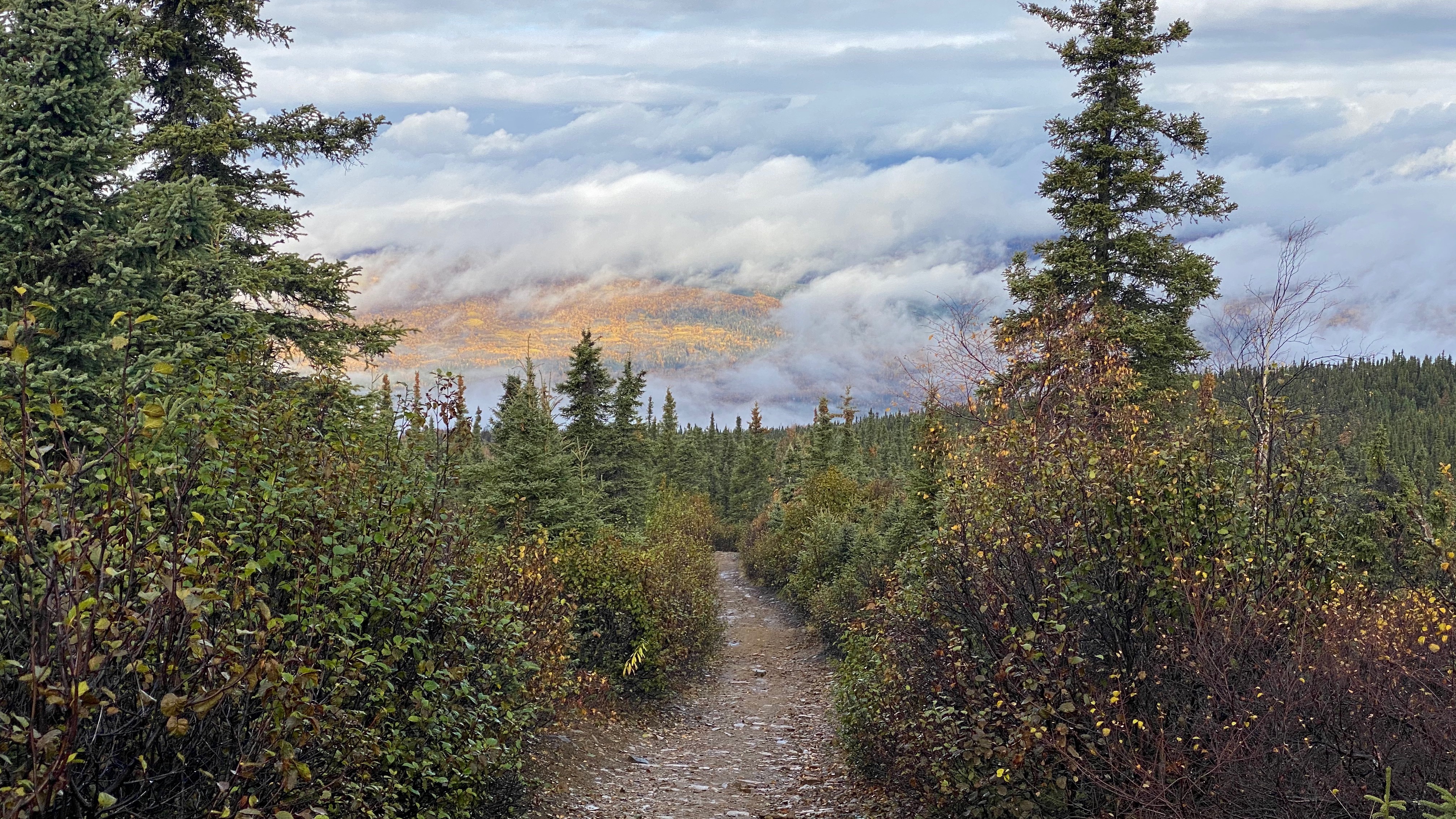
Miles 13 to 17 of the course are an out and back on a steep, rocky, and rutted four wheeler trail down the other side of Ester Dome. In a normal year, this stretch is really fun because you get a chance to cross paths with a lot of people running the race with you and get a chance to cheer people on, give high fives, and get congratulations on making it that far. At the turnaround point there’s usually a big gathering of people and a large table set out with water, sports drink, and a wide variety of food. In my cramping year two years ago, I remember relishing the pretzels on offer, and last year I ate one too many Oreo cookies on my way back up from the turnaround point. This year, it was silent and empty.
I saw a half dozen people during the out and back, and it was nice to see some of the other people that came out. For virtually the entire race, I was alone, and it felt like I was running it by myself, but this was a reminder that there were others out on the course. The back side of the Dome was below the clouds, and in the distance you could see that it was sunny down below, the turned leaves bright on the far hillside.
Out and Back
I’d been running for three hours, and matched my longest distance run of the year. For the most part, I still felt good. My right ankle and Achilles, right knee, and right hip have had issues during the year, but none of them flared up to this point. I started calculating in my head, how much time had passed and how many miles I had to go, and what sort of finish time I could expect. I decided that finishing under five hours was doable.
After the out and back the course goes along Ester Dome Road to the second relay exchange point where I’d seen Andrea and others before. Andrea refilled my water bottle again and I headed down the road to the new “chute” to the Alder Trail.
The Chute
The Alder Chute is one of the signature portions of the Equinox Course. It’s a quarter mile section of rocky trail under a power line that goes straight down Ester Dome. Straight. Down. In that quarter mile, runners descend around 350 feet. It’s so steep that just running that stretch and the Alder Trail that follows triggers deep and painful delayed onset muscle soreness (DOMS) in your quads the days following your first run down it each year no matter how fit you think you are, and it’s brutal after running 17 miles during Equinox.
Unfortunately, the Alder Chute also crosses Alaska Ski Corporation land, and runners are trespassing except on race day. A new “chute” to intersect the Alder Trail was cut this summer as part of the ITPC improvements mentioned earlier. DNR specified a similar section line easement going down the hill (south) near the intersection of Ester Dome Road and Styx River Road.
While the new Styx River chute isn’t quite as dramatic as the Alder Chute because of the switchbacks built into the trail, it still drops a similar amount of elevation over a very short distance. And it’s a much nicer trail, running through spruce forest with a thick moss layer, and occasional openings that yield views of the Tanana Valley below. I think it’ll be safer too, since it’s not as rocky and steep as the Alder Chute.
Here’s a photo from the new trail, taken in August.
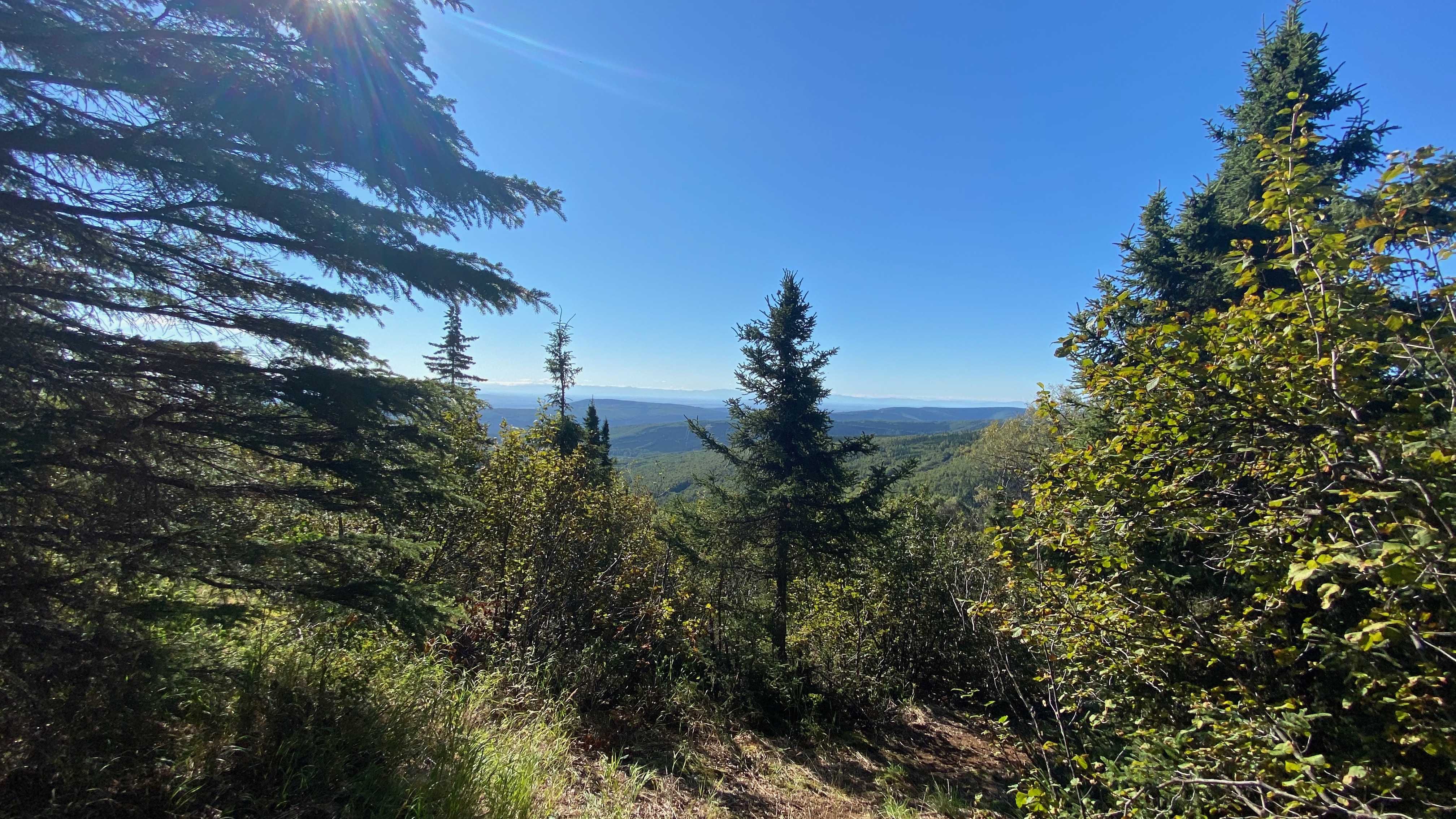
Styx River Chute, August 2020
I took it easy on this section. The trail hasn’t been worn down to mineral soil and it’s still quite steep. At one point I managed to get my foot under a root hidden under the moss and briefly lost my balance. My quads were tired from the up and down on the out and back, and I needed a breather before all the downhill running to come. Hitting the Alder Trail, which is a wider and much more established trail was a relief.
The Alder Trail
After the chute (either version) hitting the Alder Trail is always a huge relief. All the up and down of Ester Dome is over, and now the race is almost all downhill, and with a few exceptions, not super steep. The trail descends through a beautiful mixed alder and birch forest, typically in full fall colors by race day. This year, most of the leaves had fallen and were on the trail, but the birch trees lower on the trail still had their bright yellow-orange fall leaves shining at the top of the canopy. Heading back down Ester Dome, we re-entered the clouds blowing up from the valley.
On the right side of the trail in the photo you can see the metal can lid painted dark red that is the distinctive trail marker for the Equinox Course.
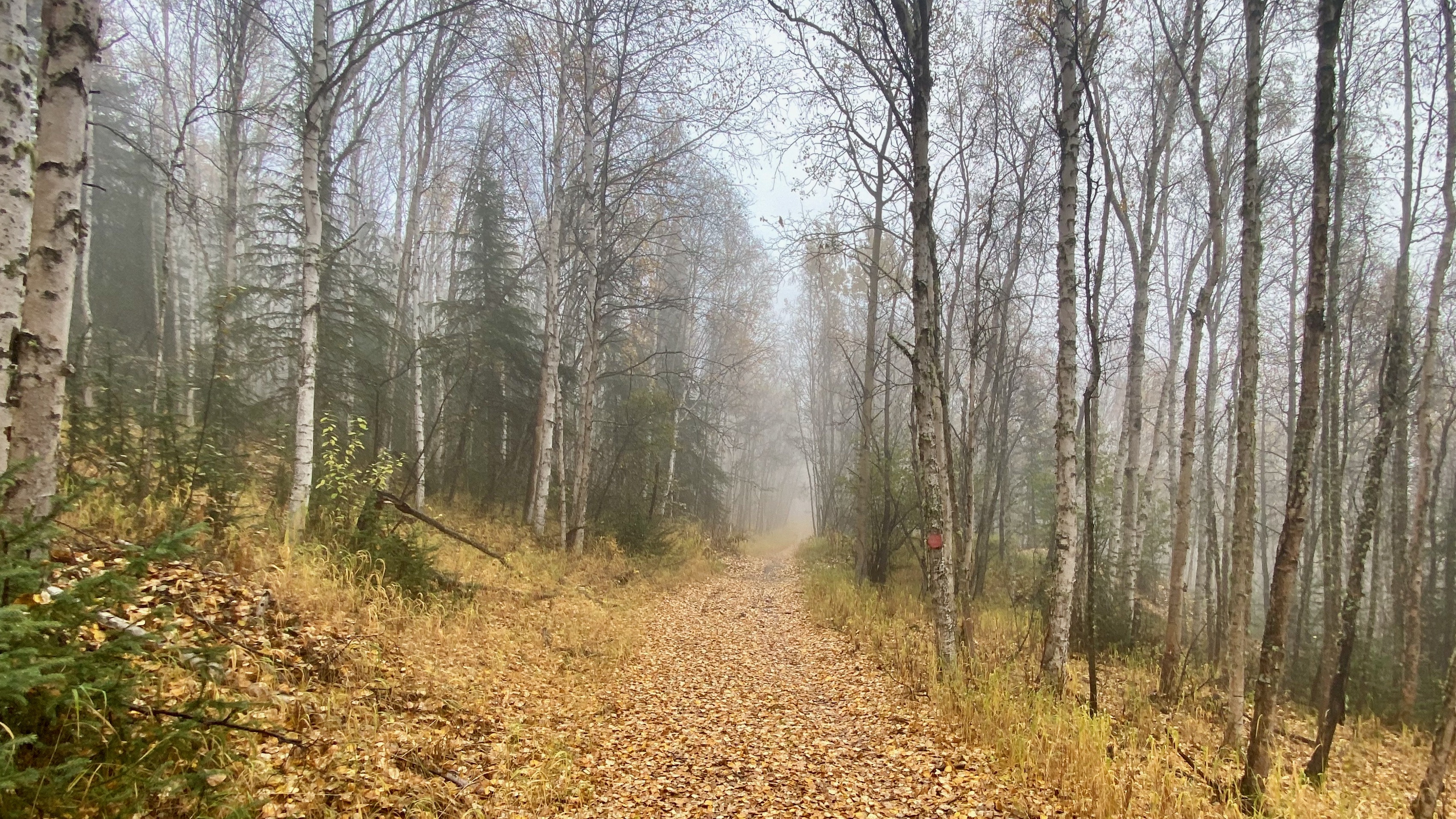
Alder Trail
Downhill running is a very different exercise from flat or uphill running and it takes practice to take advantage of it without hammering your joints. For the next four miles between miles 17 and 21, I alternated between lengthening my stride and focusing on kicking my feet up and back behind me so I wouldn’t over-stride, and shortening my stride and quickening my cadence. When my knees and feet would start feeling the effects of running hard and fast down the hill with long strides, I’d try to be light and fast on my toes to give my joints a break.
It is a falsehood to say that running damages your joints; modern evidence suggests it actually improves the condition of your joints. That said, it can be a challenge when running downhill to maintain good form, and I struggled in this stretch of the race to run a fast pace, and at the same time, keep from over-striding, dropping my hips, and letting my core relax too much. This is much more difficult after having run 20 miles and gained and lost over 3,000 feet of elevation, and I overdid it in this section of the trail. At the time, I felt great, running hard and fast on the Alder Trail to Henderson Road, but when I got there my right knee started hurting. My IT band had tightened up, causing jolts of pain in my knee when running downhill. My right hamstring was also getting closer to cramping.
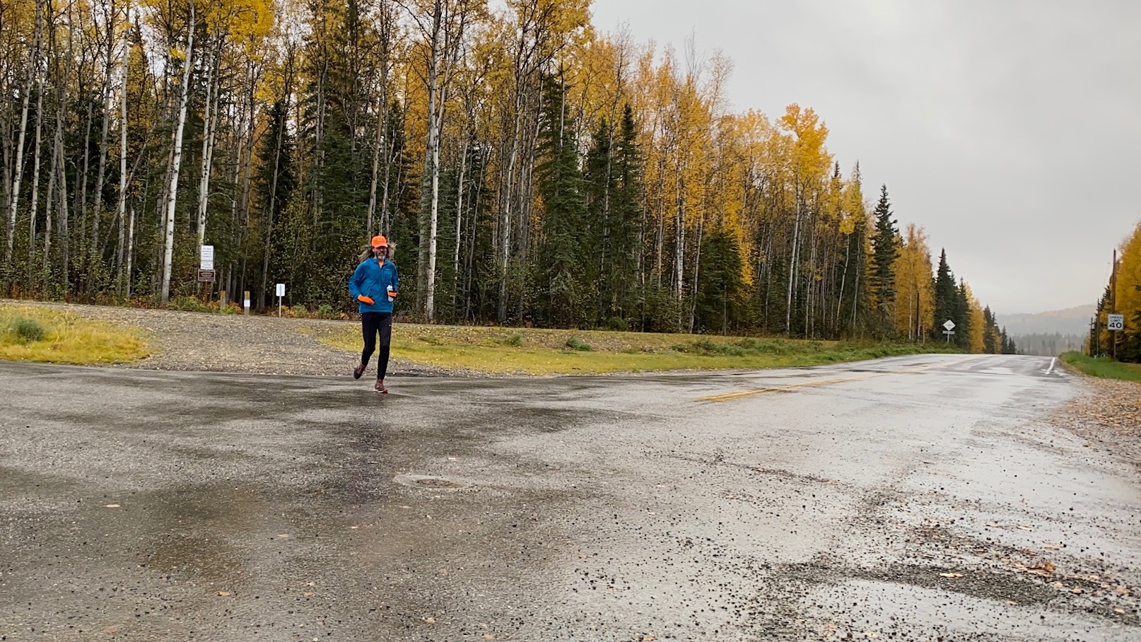
Henderson Road
From here Equinox is a mix of pavement and trail, starting with two miles of pavement along the side of Henderson Road down to the power line before Goldhill Road. At mile 20 I had my third packet of Honey Stingers, Andrea topped off my water, and I gave her my gloves and wind shirt.
On many of my training runs up and down Ester Dome, I turn left at St. Pats at this point, which leads back down to the bottom of Ester Dome Road and Ann’s Greenhouses. On race day it’s a great place to wait and watch for runners coming down the hill. Back when there was an ultra version of Equinox, runners turned onto St. Pats here and ran much of the course backwards instead of staying on Henderson.
I continued down Henderson, nursing my knee on the downhill and stopping to stretch my right hamstring occasionally. During the months leading up to the race, I ran 5-6 miles on the UAF trails three times a week, so I told myself I only had that distance left to the finish.
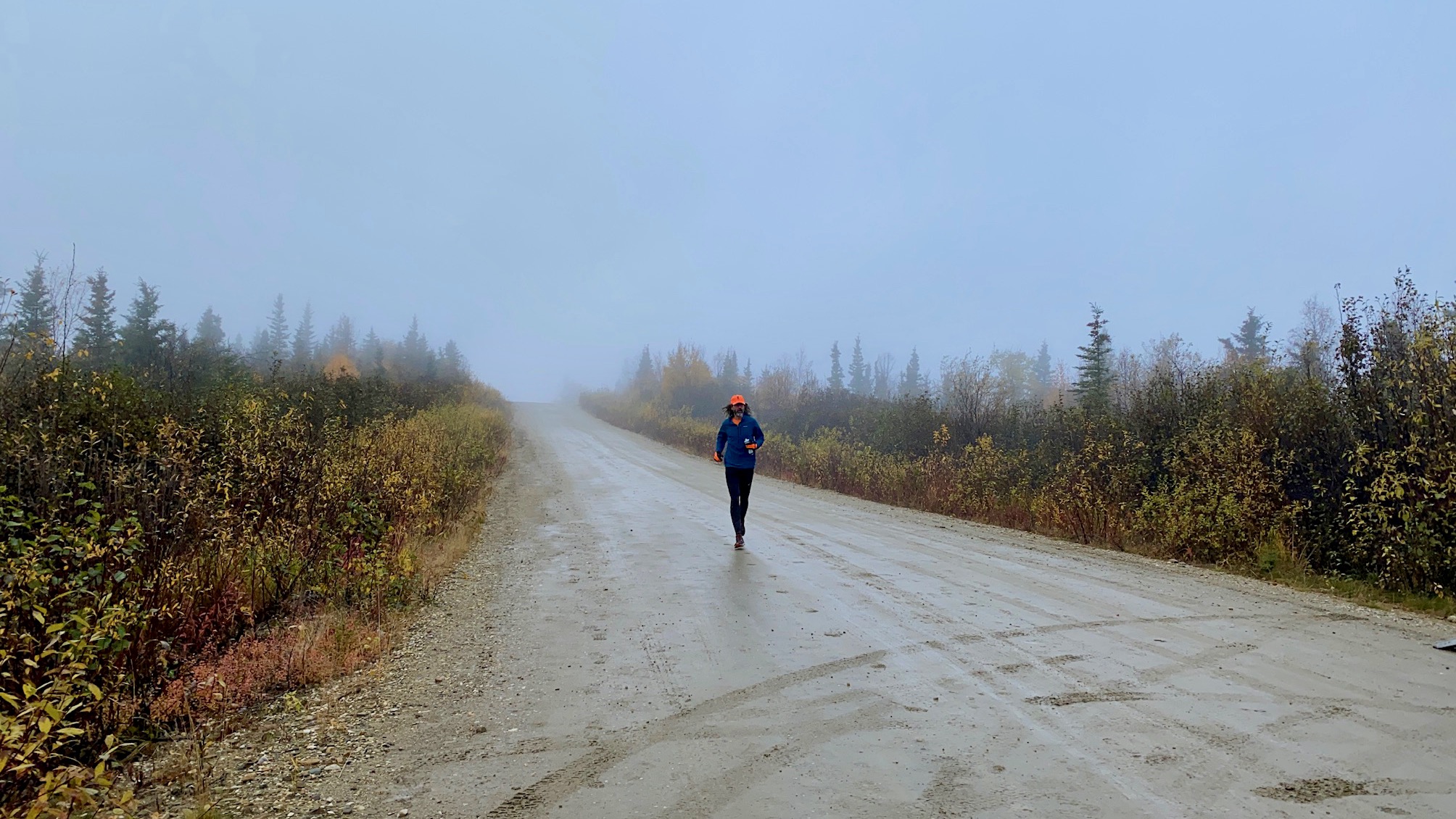
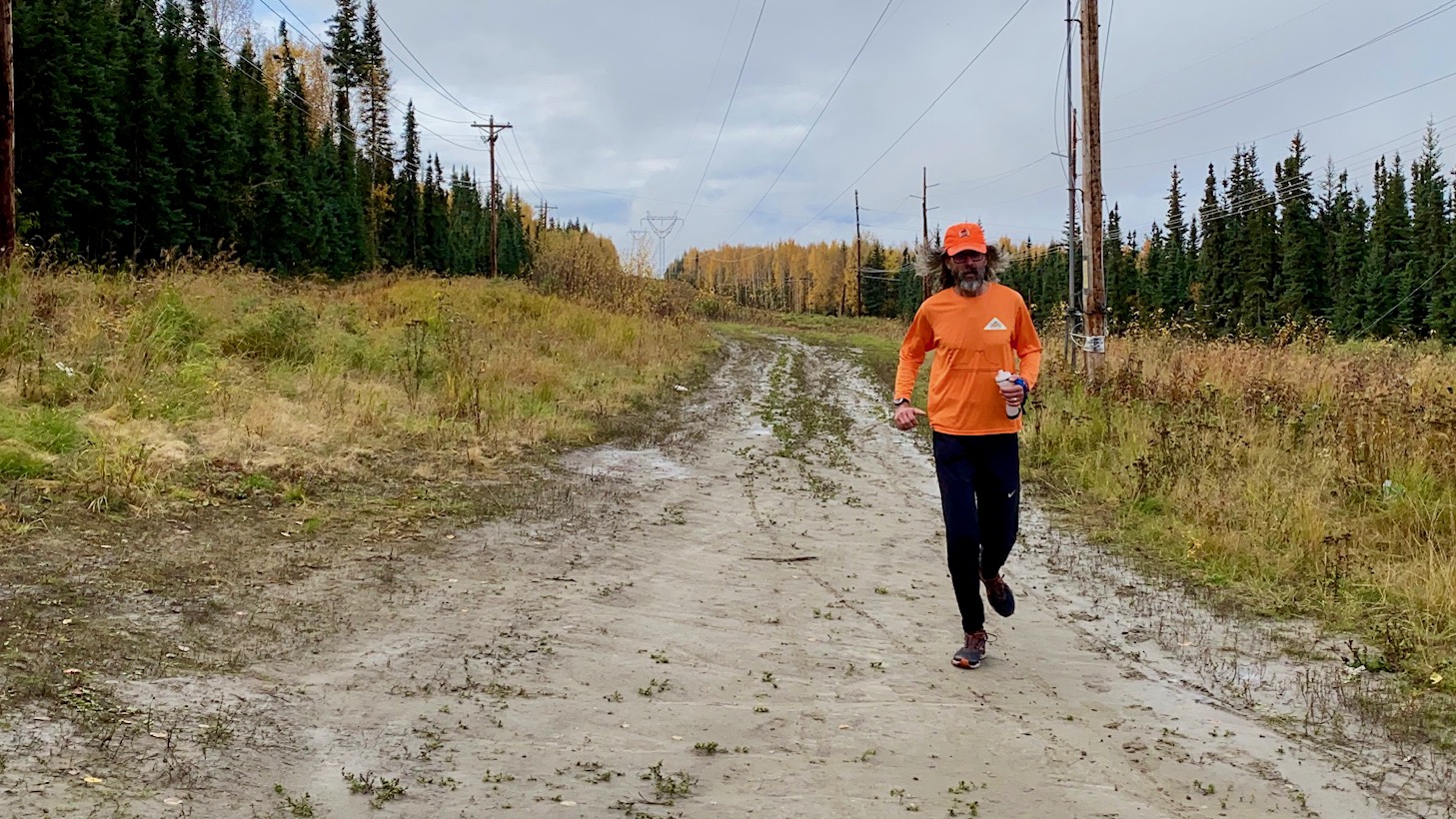
Power line and Goldhill Road
Near the end of Henderson, the trail turns left onto a wide power line that runs just north of Goldhill Road. It’s notoriously slick due to the hardpacked silt surface and late summer rain that causes a layer of algae to grow over the mud. It’s also a four wheeler track and there are a couple low spots that are deep pits of mud and water. I just barely escaped wiping out into one of these when my foot sunk into the mud and slipped backwards. The trail passes Cloudberry Lane, which is where Andrea and I got married more than twenty-three years ago. But I was only thinking of the finish line, running the uphills and trying to figure out a stride length on the downhills that reduced the pain from my IT band.
The trail slowly rises, then descends to a shallow right turn back onto Goldhill Road near the 23 mile marker. In most years, there’s a table here with salmon, drinks, and sometimes whisky. Andrea was parked there, letting me know by text that the low fork in the trail at the end was better than the upper path that is deeply rutted with four wheeler tracks.
End of the power line
For me, Goldhill road is a slog, even more so at the end of a marathon. I prefer trail running to road running, and the scenery isn’t great. You can see a long way ahead of you, reminding you of how far you have to go, and during a normal race, all the people strung out ahead of you. It being an election year, there was a diverse mix of political signs, from Quaker messages emphasizing peace and justice to one redneck yard filled with big ugly trucks and trash, flying a confederate flag.
Thankfully for my knee, it’s mostly flat, and running on roads requires a lot less concentration than trails, so it’s easier on the mind, just one foot in front of the other. I was focusing on keeping my core tight, my shoulders back, head high, and trying to stay light on my feet.
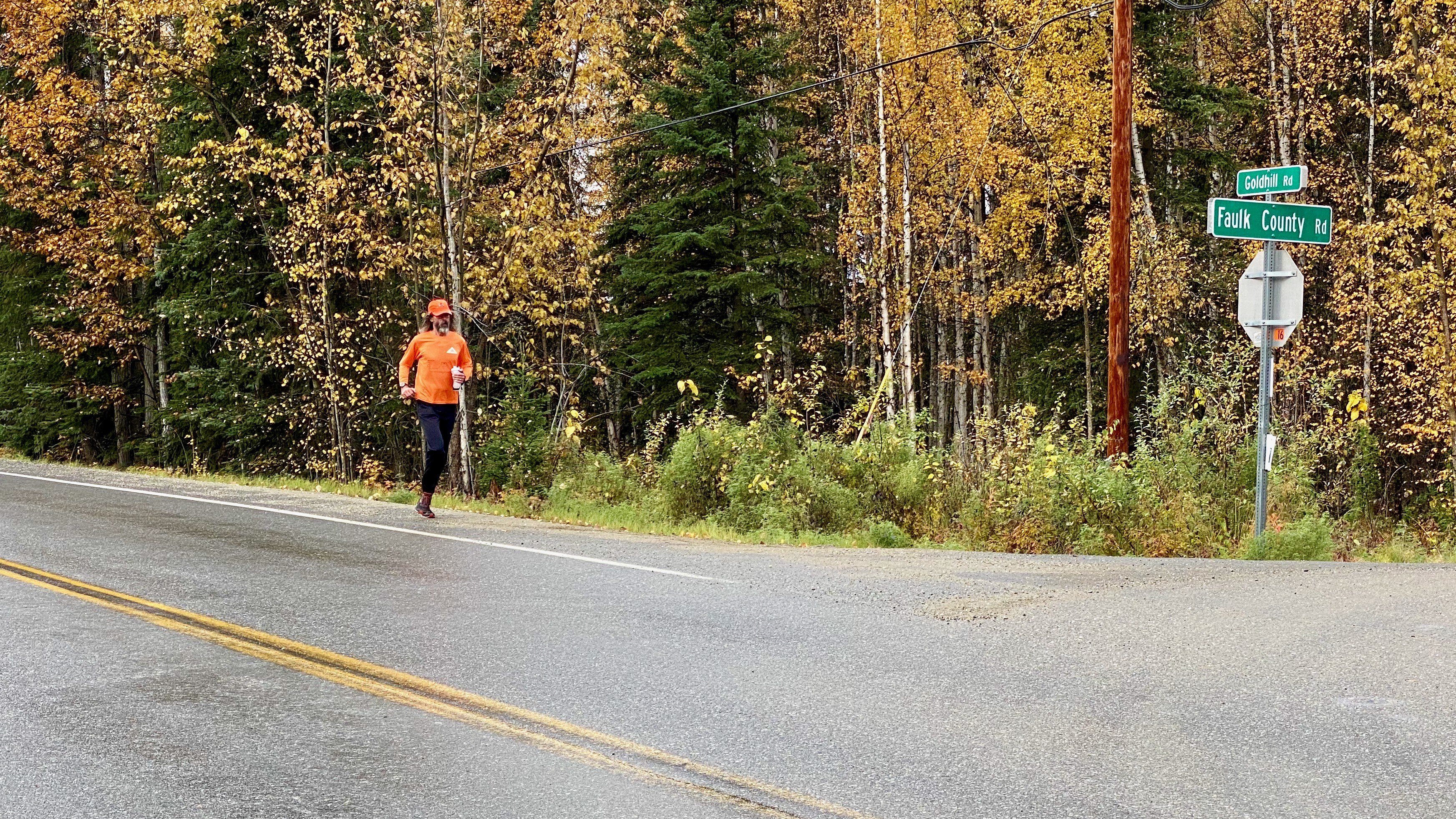
Goldhill and Faulk County
Final miles
Goldhill intersects Sheep Creek Extension, crosses the railroad tracks for the second time, turns onto Sheep Creek, and heads back onto the UAF trails for the final mile and a half to the finish line. Andrea met me on Sheep Creek Extension and we walked together for a bit before I headed up into the woods. I handed off my water bottle, checked my watch and saw I couldn’t relax if I still wanted to finish in under five hours.
Entering the trails, the course immediately goes up a short but steep hill, levels off, then goes up a much longer hill to the satellite dishes near the ski hut. It’s a killer after having run just under 25 miles, and in past years I’ve passed more than one runner walking up this section of the course. The trail comes out of the woods, crosses the road leading up to West Ridge, and heads onto the field below the Butrovich building. After a slight uphill, where I surprised a pair of walkers as I passed them, it’s all downhill to the athletic fields and the finish at Patty Center.
Last year, my legs started cramping on this last downhill, so I was careful this time as I started accelerating toward the finish line. Despite the downhill, I kept my stride long and leaned forward and my knee felt pretty good. Without an official finish line or distance, I decided to run around the outside of the field, and finish where I started at the sidewalk.
Equinox Marathon, 2020 finish
Four hours, fifty nine minutes and twenty two seconds. It’s my slowest of the four Equinox Marathons I’ve run, but it was fun, and I learned a few more things about how to run this race. Final statistics:
- 26.15 miles
- 3,599 feet of elevation gain
- 4:59:22 finish time
- 11:27 minutes/mile average pace
- Slowest mile: mile 13, 16:41 minutes/mile
- Fastest mile: mile 21, 9:43 minutes/mile
Many thanks to Andrea for being out there throughout the race. It was a lonely race where I only saw other runners for the first couple miles and during the out and back, and there was no official support so I depended on her for topping off my water and being there if I needed anything that I wasn’t carrying. She also took most of the photos in this post.
Finishing Equinox has been my goal each running season for the past several years, and I am grateful that I was able to do it again this year, despite the suck that is 2020. Very much looking forward to doing it all over again in 2021, hopefully as a real race.
Introduction
Several years ago I wrote a post about past Equinox Marathon weather. Since that post Andrea and I have run the relay twice, and I’ve run the full marathon twice. This post updates the statistics and plots to include last year’s weather data.
The official race this year was cancelled due to covid-19, but I will run it anyway, and I have no doubt many others will too. Last year’s race featured rain down in the valley, and high winds and a mixture of snow, sleet, and rain up on Ester Dome.
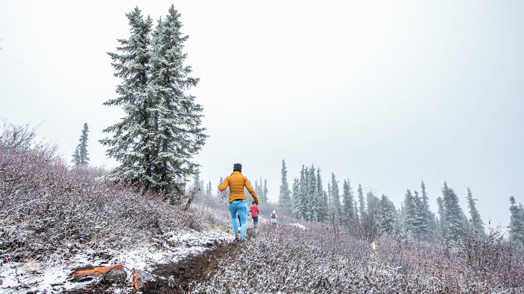
Conditions on Ester Dome during the 2019 Equinox Marathon
Methods
Methods and data are the same as in my previous post, except the daily data has been updated to include years through 2019. The R code is available at the end of the previous post.
Results
Race day weather
Temperatures at the airport on race day ranged from 19.9 °F in 1972 to 68 °F in 1969, but the average range is between 34.4 and 53.0 °F. Using our model of Ester Dome temperatures, we get an average range of 29.7 and 47.3 °F and an overall min / max of 16.1 / 61.3 °F up on the Dome. Generally speaking, it is below freezing on Ester Dome, but usually before most of the runners get up there.
Precipitation (rain, sleet or snow) has fallen on 17 out of 57 race days, or 30% of the time, and measurable snowfall has been recorded on four of those seventeen. The highest amount fell in 2014 with 0.36 inches of liquid precipitation (no snow was recorded and the temperatures were between 45 and 51 °F so it was almost certainly all rain, even on Ester Dome). More than a quarter of an inch of precipitation fell in three of the seventeen years when it rained or snowed (1990, 1993, and 2014), but most rainfall totals are much smaller.
Measurable snow fell at the airport in four years, or seven percent of the time: 4.1 inches in 1993, 2.1 inches in 1985, 1.2 inches in 1996, and 0.4 inches in 1992. But that’s at the airport station. Five of the 13 years where measurable precipitation fell at the airport and no snow fell, had possible minimum temperatures on Ester Dome that were below freezing. It’s likely that some of the precipitation recorded at the airport in those years was coming down as snow up on Ester Dome. If so, that means snow may have fallen on nine race days, bringing the percentage up to sixteen percent.
Wind data from the airport has only been recorded since 1984, but from those years the average wind speed at the airport on race day is 4.8 miles per hour. The highest 2-minute wind speed during Equinox race day was 21 miles per hour in 2003. Unfortunately, no wind data is available for Ester Dome, but it’s likely to be higher than what is recorded at the airport.
Weather from the week prior
It’s also useful to look at the weather from the week before the race, since excessive pre-race rain or snow can make conditions on race day very different, even if the race day weather is pleasant. The first year I ran the full marathon (2013), it snowed the week before and much of the trail in the woods before the water stop near Henderson and all of the out and back were covered in snow.
The most dramatic example of this was 1992 where 23 inches (!) of snow fell at the airport in the week prior to the race, with much higher totals up on the summit of Ester Dome. Measurable snow has been recorded at the airport in the week prior to six races, but all the weekly totals are under an inch except for the snow year of 1992.
Precipitation has fallen in 45 of 57 pre-race weeks (79% of the time). Three years have had more than an inch of precipitation prior to the race: 1.49 inches in 2015, 1.26 inches in 1992 (most of which fell as snow), and 1.05 inches in 2007. On average, just over two tenths of an inch of precipitation falls in the week before the race.
Summary
The following stacked plots shows the weather for all 57 runnings of the Equinox marathon. The top panel shows the range of temperatures on race day from the airport station (wide bars) and estimated on Ester Dome (thin lines below bars). The shaded area at the bottom shows where temperatures are below freezing. The orange horizonal lines represent average high and low temperature in the valley (dashed lines) and on Ester Dome (solid orange lines).
The middle panel shows race day liquid precipitation (rain, melted snow). Bars marked with an asterisk indicate years where snow was also recorded at the airport, but remember that five of the other years with liquid precipitation probably experienced snow on Ester Dome (1977, 1986, 1991, 1994, and 2016) because the temperatures were likely to be below freezing at elevation.
The bottom panel shows precipitation totals from the week prior to the race. Bars marked with an asterisk indicate weeks where snow was also recorded at the airport.

Here’s a table with most of the data from the analysis.
| Date | min t | max t | ED min t | ED max t | awnd | prcp | snow | p prcp | p snow |
|---|---|---|---|---|---|---|---|---|---|
| 1963-09-21 | 32.0 | 54.0 | 27.5 | 48.2 | 0.00 | 0.0 | 0.01 | 0.0 | |
| 1964-09-19 | 34.0 | 57.9 | 29.4 | 51.8 | 0.00 | 0.0 | 0.03 | 0.0 | |
| 1965-09-25 | 37.9 | 60.1 | 33.1 | 53.9 | 0.00 | 0.0 | 0.80 | 0.0 | |
| 1966-09-24 | 36.0 | 62.1 | 31.3 | 55.8 | 0.00 | 0.0 | 0.01 | 0.0 | |
| 1967-09-23 | 35.1 | 57.9 | 30.4 | 51.8 | 0.00 | 0.0 | 0.00 | 0.0 | |
| 1968-09-21 | 23.0 | 44.1 | 19.1 | 38.9 | 0.00 | 0.0 | 0.04 | 0.0 | |
| 1969-09-20 | 35.1 | 68.0 | 30.4 | 61.3 | 0.00 | 0.0 | 0.00 | 0.0 | |
| 1970-09-19 | 24.1 | 39.9 | 20.1 | 34.9 | 0.00 | 0.0 | 0.42 | 0.0 | |
| 1971-09-18 | 35.1 | 55.9 | 30.4 | 50.0 | 0.00 | 0.0 | 0.14 | 0.0 | |
| 1972-09-23 | 19.9 | 42.1 | 16.1 | 37.0 | 0.00 | 0.0 | 0.01 | 0.2 | |
| 1973-09-22 | 30.0 | 44.1 | 25.6 | 38.9 | 0.00 | 0.0 | 0.05 | 0.0 | |
| 1974-09-21 | 48.0 | 60.1 | 42.5 | 53.9 | 0.08 | 0.0 | 0.00 | 0.0 | |
| 1975-09-20 | 37.9 | 55.9 | 33.1 | 50.0 | 0.02 | 0.0 | 0.02 | 0.0 | |
| 1976-09-18 | 34.0 | 59.0 | 29.4 | 52.9 | 0.00 | 0.0 | 0.54 | 0.0 | |
| 1977-09-24 | 36.0 | 48.9 | 31.3 | 43.4 | 0.06 | 0.0 | 0.20 | 0.0 | |
| 1978-09-23 | 30.0 | 42.1 | 25.6 | 37.0 | 0.00 | 0.0 | 0.10 | 0.3 | |
| 1979-09-22 | 35.1 | 62.1 | 30.4 | 55.8 | 0.00 | 0.0 | 0.17 | 0.0 | |
| 1980-09-20 | 30.9 | 43.0 | 26.5 | 37.8 | 0.00 | 0.0 | 0.35 | 0.0 | |
| 1981-09-19 | 37.0 | 43.0 | 32.2 | 37.8 | 0.15 | 0.0 | 0.04 | 0.0 | |
| 1982-09-18 | 42.1 | 61.0 | 37.0 | 54.8 | 0.02 | 0.0 | 0.22 | 0.0 | |
| 1983-09-17 | 39.9 | 46.9 | 34.9 | 41.5 | 0.00 | 0.0 | 0.05 | 0.0 | |
| 1984-09-22 | 28.9 | 60.1 | 24.6 | 53.9 | 5.8 | 0.00 | 0.0 | 0.08 | 0.0 |
| 1985-09-21 | 30.9 | 42.1 | 26.5 | 37.0 | 6.5 | 0.14 | 2.1 | 0.57 | 0.0 |
| 1986-09-20 | 36.0 | 52.0 | 31.3 | 46.3 | 8.3 | 0.07 | 0.0 | 0.21 | 0.0 |
| 1987-09-19 | 37.9 | 61.0 | 33.1 | 54.8 | 6.3 | 0.00 | 0.0 | 0.00 | 0.0 |
| 1988-09-24 | 37.0 | 45.0 | 32.2 | 39.7 | 4.0 | 0.00 | 0.0 | 0.11 | 0.0 |
| 1989-09-23 | 36.0 | 61.0 | 31.3 | 54.8 | 8.5 | 0.00 | 0.0 | 0.07 | 0.5 |
| 1990-09-22 | 37.9 | 50.0 | 33.1 | 44.4 | 7.8 | 0.26 | 0.0 | 0.00 | 0.0 |
| 1991-09-21 | 36.0 | 57.0 | 31.3 | 51.0 | 4.5 | 0.04 | 0.0 | 0.03 | 0.0 |
| 1992-09-19 | 24.1 | 33.1 | 20.1 | 28.5 | 6.7 | 0.01 | 0.4 | 1.26 | 23.0 |
| 1993-09-18 | 28.0 | 37.0 | 23.8 | 32.2 | 4.9 | 0.29 | 4.1 | 0.37 | 0.3 |
| 1994-09-24 | 27.0 | 51.1 | 22.8 | 45.5 | 6.0 | 0.02 | 0.0 | 0.08 | 0.0 |
| 1995-09-23 | 43.0 | 66.9 | 37.8 | 60.3 | 4.0 | 0.00 | 0.0 | 0.00 | 0.0 |
| 1996-09-21 | 28.9 | 37.9 | 24.6 | 33.1 | 6.9 | 0.06 | 1.2 | 0.26 | 0.0 |
| 1997-09-20 | 27.0 | 55.0 | 22.8 | 49.1 | 3.8 | 0.00 | 0.0 | 0.03 | 0.0 |
| 1998-09-19 | 42.1 | 60.1 | 37.0 | 53.9 | 4.9 | 0.00 | 0.0 | 0.37 | 0.0 |
| 1999-09-18 | 39.0 | 64.9 | 34.1 | 58.4 | 3.8 | 0.00 | 0.0 | 0.26 | 0.0 |
| 2000-09-16 | 28.9 | 50.0 | 24.6 | 44.4 | 5.6 | 0.00 | 0.0 | 0.30 | 0.0 |
| 2001-09-22 | 33.1 | 57.0 | 28.5 | 51.0 | 1.6 | 0.00 | 0.0 | 0.00 | 0.0 |
| 2002-09-21 | 33.1 | 48.9 | 28.5 | 43.4 | 3.8 | 0.00 | 0.0 | 0.03 | 0.0 |
| 2003-09-20 | 26.1 | 46.0 | 22.0 | 40.7 | 9.6 | 0.00 | 0.0 | 0.00 | 0.0 |
| 2004-09-18 | 26.1 | 48.0 | 22.0 | 42.5 | 4.3 | 0.00 | 0.0 | 0.25 | 0.0 |
| 2005-09-17 | 37.0 | 63.0 | 32.2 | 56.6 | 0.9 | 0.00 | 0.0 | 0.09 | 0.0 |
| 2006-09-16 | 46.0 | 64.0 | 40.7 | 57.6 | 4.3 | 0.00 | 0.0 | 0.00 | 0.0 |
| 2007-09-22 | 25.0 | 45.0 | 20.9 | 39.7 | 4.7 | 0.00 | 0.0 | 1.05 | 0.0 |
| 2008-09-20 | 34.0 | 51.1 | 29.4 | 45.5 | 4.5 | 0.00 | 0.0 | 0.08 | 0.0 |
| 2009-09-19 | 39.0 | 50.0 | 34.1 | 44.4 | 5.8 | 0.00 | 0.0 | 0.25 | 0.0 |
| 2010-09-18 | 35.1 | 64.9 | 30.4 | 58.4 | 2.5 | 0.00 | 0.0 | 0.00 | 0.0 |
| 2011-09-17 | 39.9 | 57.9 | 34.9 | 51.8 | 1.3 | 0.00 | 0.0 | 0.44 | 0.0 |
| 2012-09-22 | 46.9 | 66.9 | 41.5 | 60.3 | 6.0 | 0.00 | 0.0 | 0.33 | 0.0 |
| 2013-09-21 | 24.3 | 44.1 | 20.3 | 38.9 | 5.1 | 0.00 | 0.0 | 0.13 | 0.6 |
| 2014-09-20 | 45.0 | 51.1 | 39.7 | 45.5 | 1.6 | 0.36 | 0.0 | 0.00 | 0.0 |
| 2015-09-19 | 37.9 | 44.1 | 33.1 | 38.9 | 2.9 | 0.01 | 0.0 | 1.49 | 0.0 |
| 2016-09-17 | 34.0 | 57.9 | 29.4 | 51.8 | 2.2 | 0.01 | 0.0 | 0.61 | 0.0 |
| 2017-09-16 | 33.1 | 66.0 | 28.5 | 59.5 | 3.1 | 0.00 | 0.0 | 0.02 | 0.0 |
| 2018-09-15 | 44.1 | 60.1 | 38.9 | 53.9 | 3.8 | 0.00 | 0.0 | 0.00 | 0.0 |
| 2019-09-21 | 37.0 | 45.0 | 32.2 | 39.7 | 7.6 | 0.13 | 0.0 | 0.40 | 0.0 |
Introduction
At the 57th running of the Equinox Marathon last weekend Aaron Fletcher broke Stan Justice’s 1985 course record, one of the oldest running records in Alaska sports. On the Equinox Marathon Facebook page Stan and Matias Saari were discussing whether more favorable weather might have meant an even faster record-breaking effort. Stan writes:
Where is a statistician when you need one. Would be interesting to compare times of all 2018 runners with their 2019 times.
I’m not a statistician, but let’s take a look.
Results
We’ve got Equinox Marathon finish time data going back to 1997, so we’ll compare the finish times for all runners who competed in consecutive years, subtracting their current year finish times (in hours) from the previous year. By this metric, negative values indicate individuals who ran faster in the current year than the previous. For example, I completed the race in 4:40:05 in 2018, and finished in 4:33:42 this year. My “hours_delta” for 2019 is -0.106 hours, or 6 minutes, 23 seconds faster.
Here’s the distribution of this statistic for 2019:

There are several people who were dramatically faster (on the left side of the graph), but the overall picture shows that times in 2019 were slower than 2018. The dark cyan line is the median value, which is at 0.18 hours or 10 minutes, 35 seconds slower. There were 53 runners that ran the race faster in 2019 than 2018 (including me), and 115 who were slower. That’s a pretty dramatic difference.
Here’s that relationship for all the years where we have data:

The orange bars are runners who ran that year’s Equinox faster than the previous year and the dark cyan bars are those who were slower. 2019 is dramatically different than most other years for how much slower most people ran. 2013 is another particularly slow year. Fast years include 2007, 2009, and last year.
Here’s another way to look at the data. It shows the median number of minutes runners ran Equinox faster (negative numbers) or slower (positive) in consecutive years.

You can see that finish times were dramatically slower in 2019, and much faster in 2018. Since this comparison is using paired comparisons between years, at least part of the reason 2019 seemed like such a slow race is that 2018 was a fast one.
Two-year lag
Let’s see what happens if we use a two-year lag to calculate the differences. Instead of comparing the current year’s results with the previous year for individual runners that raced in both years, we’ll compare the current year with two years prior. For example runners that ran the race this year and in 2017.
Here’s what the distribution looks like comparing 2019 and 2017 results from the same runner.

It’s a similar pattern, with the median values at 0.18 hours, indicating that runners were almost 10 minutes slower in 2019 when compared against their 2017 times. This strengthens the evidence that 2019 was a particularly difficult year to run the race.
Median difference by year for all years of the two-year lag data:

Remember that the dark cyan bars are years with slower finish times and orange are faster. 2019 still comes out as an outlier, along with 2013. 2007 is the clear winner for fast times.
All pairwise race results
If we can do one and two year lags, how about combining all the pairwise race results? At some point the comparison is no longer a good one because of the large time interval between races, so we will restrict the comparisons to six or fewer years between results. We’ll also remove the earliest years from the results because those years are likely biased by having fewer long lag results.
Here’s the same plot showing difference times in minutes for all pairwise race results, six years and fewer.

You can see that there’s a pretty strong bias toward slower times, which is likely due to people aging and their times getting slower. The conditions were good enough in 2007 that this aging effect was offset and people running in that race tended to do it faster than their earlier performances despite being older. Even so, 2019 still stands out as one of the most difficult races.
Here’s the aging effect:
##
## Call:
## lm(formula = hours_delta ~ years_delta, data = all_through_six)
##
## Residuals:
##     Min      1Q  Median      3Q     Max
## -6.3242 -0.3639 -0.0415  0.3115  6.4441
##
## Coefficients:
##             Estimate Std. Error t value            Pr(>|t|)
## (Intercept) -0.03390    0.01934  -1.752              0.0797 .
## years_delta  0.05152    0.00558   9.234 <0.0000000000000002 ***
## ---
## Signif. codes:  0 '***' 0.001 '**' 0.01 '*' 0.05 '.' 0.1 ' ' 1
##
## Residual standard error: 0.8845 on 8664 degrees of freedom
## Multiple R-squared:  0.009745,   Adjusted R-squared:  0.00963
## F-statistic: 85.26 on 1 and 8664 DF,  p-value: < 0.00000000000000022
There’s a very significant positive relationship between the difference in years and the difference in marathon times for those runners (years_delta in the coefficient results above). The longer the gap between races, the slower a runner is by just over 3 minutes each year. Notice, however, that the noise in the data is so great that this model, no matter how significant the coefficients, explains almost none of the variation in the difference in marathon times (dismally small R-squared values).
Weather
The conditions in this year’s race were particularly harsh with a fairly constant 40 °F temperature and light rain falling at valley level; and below freezing temperatures, high winds, and snow falling up on Ester Dome. The trail was muddy, soft, and slippery in places, especially the single track and the on the unpaved section of Henderson Road. Compare this with last year when the weather was gorgeous: dry, sunny, and temperatures ranging from 39—60 °F.
We took a look at the differences in weather between years to see if there is a relationship between weather differences and finish time differences, but none of the models we tried were any good at predicting differences in finish times, probably because of the huge variation in finish times that had nothing to do with the weather. There are too many other factors contributing to an individual’s performance from one year to the next to be able to pull out just the effects of weather on the results.
Conclusion
2019 was a very slow year when we compared runners who completed Equinox in 2019 and earlier years. In fact, there’s some evidence that it’s the slowest year of all the years considered here (1997—2019). We could find no statistical evidence to show that weather was the cause of this, but anyone who was out there on race day this year knows it played a part in their finish times. I ran the race this year and last and managed to improve on my time despite the conditions, but I don’t think there’s any question that I would have improved my time even more had it been warm and sunny instead of cold, windy, and wet. Congratulations to all the competitors in this year’s race. It was a fun, but challenging year for Equinox.
Introduction
A couple years ago I wrote a post about past Equinox Marathon weather. Since that post Andrea and I have run the relay twice, and I ran the full marathon. This post updates the statistics and plots to include two more years of the race.
Methods
Methods and data are the same as in my previous post, except the daily data has been updated to include 2018. The R code is available at the end of the previous post.
Results
Race day weather
Temperatures at the airport on race day ranged from 19.9 °F in 1972 to 35.1 °F in 1969, but the average range is between 34.3 and 53.2 °F. Using our model of Ester Dome temperatures, we get an average range of 29.7 and 47.4 °F and an overall min / max of 16.1 / 61.3 °F. Generally speaking, it will be below freezing on Ester Dome, but possibly before most of the runners get up there.
Precipitation (rain, sleet or snow) has fallen on 16 out of 56 race days, or 29% of the time, and measurable snowfall has been recorded on four of those sixteen. The highest amount fell in 2014 with 0.36 inches of liquid precipitation (no snow was recorded and the temperatures were between 45 and 51 °F so it was almost certainly all rain, even on Ester Dome). More than a quarter of an inch of precipitation fell in three of the sixteen years when it rained or snowed (1990, 1993, and 2014), but most rainfall totals are much smaller.
Measurable snow fell at the airport in four years, or seven percent of the time: 4.1 inches in 1993, 2.1 inches in 1985, 1.2 inches in 1996, and 0.4 inches in 1992. But that’s at the airport station. Five of the 12 years where measurable precipitation fell at the airport and no snow fell, had possible minimum temperatures on Ester Dome that were below freezing. It’s likely that some of the precipitation recorded at the airport in those years was coming down as snow up on Ester Dome. If so, that means snow may have fallen on nine race days, bringing the percentage up to sixteen percent.
Wind data from the airport has only been recorded since 1984, but from those years the average wind speed at the airport on race day is 4.8 miles per hour. The highest 2-minute wind speed during Equinox race day was 21 miles per hour in 2003. Unfortunately, no wind data is available for Ester Dome, but it’s likely to be higher than what is recorded at the airport.
Weather from the week prior
It’s also useful to look at the weather from the week before the race, since excessive pre-race rain or snow can make conditions on race day very different, even if the race day weather is pleasant. The year I ran the full marathon (2013), it snowed the week before and much of the trail in the woods before the water stop near Henderson and all of the out and back were covered in snow.
The most dramatic example of this was 1992 where 23 inches (!) of snow fell at the airport in the week prior to the race, with much higher totals up on the summit of Ester Dome. Measurable snow has been recorded at the airport in the week prior to six races, but all the weekly totals are under an inch except for the snow year of 1992.
Precipitation has fallen in 44 of 56 pre-race weeks (79% of the time). Three years have had more than an inch of precipitation prior to the race: 1.49 inches in 2015, 1.26 inches in 1992 (most of which fell as snow), and 1.05 inches in 2007. On average, just over two tenths of an inch of precipitation falls in the week before the race.
Summary
The following stacked plots shows the weather for all 56 runnings of the Equinox marathon. The top panel shows the range of temperatures on race day from the airport station (wide bars) and estimated on Ester Dome (thin lines below bars). The shaded area at the bottom shows where temperatures are below freezing.
The middle panel shows race day liquid precipitation (rain, melted snow). Bars marked with an asterisk indicate years where snow was also recorded at the airport, but remember that five of the other years with liquid precipitation probably experienced snow on Ester Dome (1977, 1986, 1991, 1994, and 2016) because the temperatures were likely to be below freezing at elevation.
The bottom panel shows precipitation totals from the week prior to the race. Bars marked with an asterisk indicate weeks where snow was also recorded at the airport.

Here’s a table with most of the data from the analysis. A CSV with this data can be downloaded from all_wx.csv
| Date | min t | max t | ED min t | ED max t | awnd | prcp | snow | p prcp | p snow |
|---|---|---|---|---|---|---|---|---|---|
| 1963-09-21 | 32.0 | 54.0 | 27.5 | 48.2 | 0.00 | 0.0 | 0.01 | 0.0 | |
| 1964-09-19 | 34.0 | 57.9 | 29.4 | 51.8 | 0.00 | 0.0 | 0.03 | 0.0 | |
| 1965-09-25 | 37.9 | 60.1 | 33.1 | 53.9 | 0.00 | 0.0 | 0.80 | 0.0 | |
| 1966-09-24 | 36.0 | 62.1 | 31.3 | 55.8 | 0.00 | 0.0 | 0.01 | 0.0 | |
| 1967-09-23 | 35.1 | 57.9 | 30.4 | 51.8 | 0.00 | 0.0 | 0.00 | 0.0 | |
| 1968-09-21 | 23.0 | 44.1 | 19.1 | 38.9 | 0.00 | 0.0 | 0.04 | 0.0 | |
| 1969-09-20 | 35.1 | 68.0 | 30.4 | 61.3 | 0.00 | 0.0 | 0.00 | 0.0 | |
| 1970-09-19 | 24.1 | 39.9 | 20.1 | 34.9 | 0.00 | 0.0 | 0.42 | 0.0 | |
| 1971-09-18 | 35.1 | 55.9 | 30.4 | 50.0 | 0.00 | 0.0 | 0.14 | 0.0 | |
| 1972-09-23 | 19.9 | 42.1 | 16.1 | 37.0 | 0.00 | 0.0 | 0.01 | 0.2 | |
| 1973-09-22 | 30.0 | 44.1 | 25.6 | 38.9 | 0.00 | 0.0 | 0.05 | 0.0 | |
| 1974-09-21 | 48.0 | 60.1 | 42.5 | 53.9 | 0.08 | 0.0 | 0.00 | 0.0 | |
| 1975-09-20 | 37.9 | 55.9 | 33.1 | 50.0 | 0.02 | 0.0 | 0.02 | 0.0 | |
| 1976-09-18 | 34.0 | 59.0 | 29.4 | 52.9 | 0.00 | 0.0 | 0.54 | 0.0 | |
| 1977-09-24 | 36.0 | 48.9 | 31.3 | 43.4 | 0.06 | 0.0 | 0.20 | 0.0 | |
| 1978-09-23 | 30.0 | 42.1 | 25.6 | 37.0 | 0.00 | 0.0 | 0.10 | 0.3 | |
| 1979-09-22 | 35.1 | 62.1 | 30.4 | 55.8 | 0.00 | 0.0 | 0.17 | 0.0 | |
| 1980-09-20 | 30.9 | 43.0 | 26.5 | 37.8 | 0.00 | 0.0 | 0.35 | 0.0 | |
| 1981-09-19 | 37.0 | 43.0 | 32.2 | 37.8 | 0.15 | 0.0 | 0.04 | 0.0 | |
| 1982-09-18 | 42.1 | 61.0 | 37.0 | 54.8 | 0.02 | 0.0 | 0.22 | 0.0 | |
| 1983-09-17 | 39.9 | 46.9 | 34.9 | 41.5 | 0.00 | 0.0 | 0.05 | 0.0 | |
| 1984-09-22 | 28.9 | 60.1 | 24.6 | 53.9 | 5.8 | 0.00 | 0.0 | 0.08 | 0.0 |
| 1985-09-21 | 30.9 | 42.1 | 26.5 | 37.0 | 6.5 | 0.14 | 2.1 | 0.57 | 0.0 |
| 1986-09-20 | 36.0 | 52.0 | 31.3 | 46.3 | 8.3 | 0.07 | 0.0 | 0.21 | 0.0 |
| 1987-09-19 | 37.9 | 61.0 | 33.1 | 54.8 | 6.3 | 0.00 | 0.0 | 0.00 | 0.0 |
| 1988-09-24 | 37.0 | 45.0 | 32.2 | 39.7 | 4.0 | 0.00 | 0.0 | 0.11 | 0.0 |
| 1989-09-23 | 36.0 | 61.0 | 31.3 | 54.8 | 8.5 | 0.00 | 0.0 | 0.07 | 0.5 |
| 1990-09-22 | 37.9 | 50.0 | 33.1 | 44.4 | 7.8 | 0.26 | 0.0 | 0.00 | 0.0 |
| 1991-09-21 | 36.0 | 57.0 | 31.3 | 51.0 | 4.5 | 0.04 | 0.0 | 0.03 | 0.0 |
| 1992-09-19 | 24.1 | 33.1 | 20.1 | 28.5 | 6.7 | 0.01 | 0.4 | 1.26 | 23.0 |
| 1993-09-18 | 28.0 | 37.0 | 23.8 | 32.2 | 4.9 | 0.29 | 4.1 | 0.37 | 0.3 |
| 1994-09-24 | 27.0 | 51.1 | 22.8 | 45.5 | 6.0 | 0.02 | 0.0 | 0.08 | 0.0 |
| 1995-09-23 | 43.0 | 66.9 | 37.8 | 60.3 | 4.0 | 0.00 | 0.0 | 0.00 | 0.0 |
| 1996-09-21 | 28.9 | 37.9 | 24.6 | 33.1 | 6.9 | 0.06 | 1.2 | 0.26 | 0.0 |
| 1997-09-20 | 27.0 | 55.0 | 22.8 | 49.1 | 3.8 | 0.00 | 0.0 | 0.03 | 0.0 |
| 1998-09-19 | 42.1 | 60.1 | 37.0 | 53.9 | 4.9 | 0.00 | 0.0 | 0.37 | 0.0 |
| 1999-09-18 | 39.0 | 64.9 | 34.1 | 58.4 | 3.8 | 0.00 | 0.0 | 0.26 | 0.0 |
| 2000-09-16 | 28.9 | 50.0 | 24.6 | 44.4 | 5.6 | 0.00 | 0.0 | 0.30 | 0.0 |
| 2001-09-22 | 33.1 | 57.0 | 28.5 | 51.0 | 1.6 | 0.00 | 0.0 | 0.00 | 0.0 |
| 2002-09-21 | 33.1 | 48.9 | 28.5 | 43.4 | 3.8 | 0.00 | 0.0 | 0.03 | 0.0 |
| 2003-09-20 | 26.1 | 46.0 | 22.0 | 40.7 | 9.6 | 0.00 | 0.0 | 0.00 | 0.0 |
| 2004-09-18 | 26.1 | 48.0 | 22.0 | 42.5 | 4.3 | 0.00 | 0.0 | 0.25 | 0.0 |
| 2005-09-17 | 37.0 | 63.0 | 32.2 | 56.6 | 0.9 | 0.00 | 0.0 | 0.09 | 0.0 |
| 2006-09-16 | 46.0 | 64.0 | 40.7 | 57.6 | 4.3 | 0.00 | 0.0 | 0.00 | 0.0 |
| 2007-09-22 | 25.0 | 45.0 | 20.9 | 39.7 | 4.7 | 0.00 | 0.0 | 1.05 | 0.0 |
| 2008-09-20 | 34.0 | 51.1 | 29.4 | 45.5 | 4.5 | 0.00 | 0.0 | 0.08 | 0.0 |
| 2009-09-19 | 39.0 | 50.0 | 34.1 | 44.4 | 5.8 | 0.00 | 0.0 | 0.25 | 0.0 |
| 2010-09-18 | 35.1 | 64.9 | 30.4 | 58.4 | 2.5 | 0.00 | 0.0 | 0.00 | 0.0 |
| 2011-09-17 | 39.9 | 57.9 | 34.9 | 51.8 | 1.3 | 0.00 | 0.0 | 0.44 | 0.0 |
| 2012-09-22 | 46.9 | 66.9 | 41.5 | 60.3 | 6.0 | 0.00 | 0.0 | 0.33 | 0.0 |
| 2013-09-21 | 24.3 | 44.1 | 20.3 | 38.9 | 5.1 | 0.00 | 0.0 | 0.13 | 0.6 |
| 2014-09-20 | 45.0 | 51.1 | 39.7 | 45.5 | 1.6 | 0.36 | 0.0 | 0.00 | 0.0 |
| 2015-09-19 | 37.9 | 44.1 | 33.1 | 38.9 | 2.9 | 0.01 | 0.0 | 1.49 | 0.0 |
| 2016-09-17 | 34.0 | 57.9 | 29.4 | 51.8 | 2.2 | 0.01 | 0.0 | 0.61 | 0.0 |
| 2017-09-16 | 33.1 | 66.0 | 28.5 | 59.5 | 3.1 | 0.00 | 0.0 | 0.02 | 0.0 |
| 2018-09-15 | 44.1 | 60.1 | 38.9 | 53.9 | 3.8 | 0.00 | 0.0 | 0.00 | 0.0 |
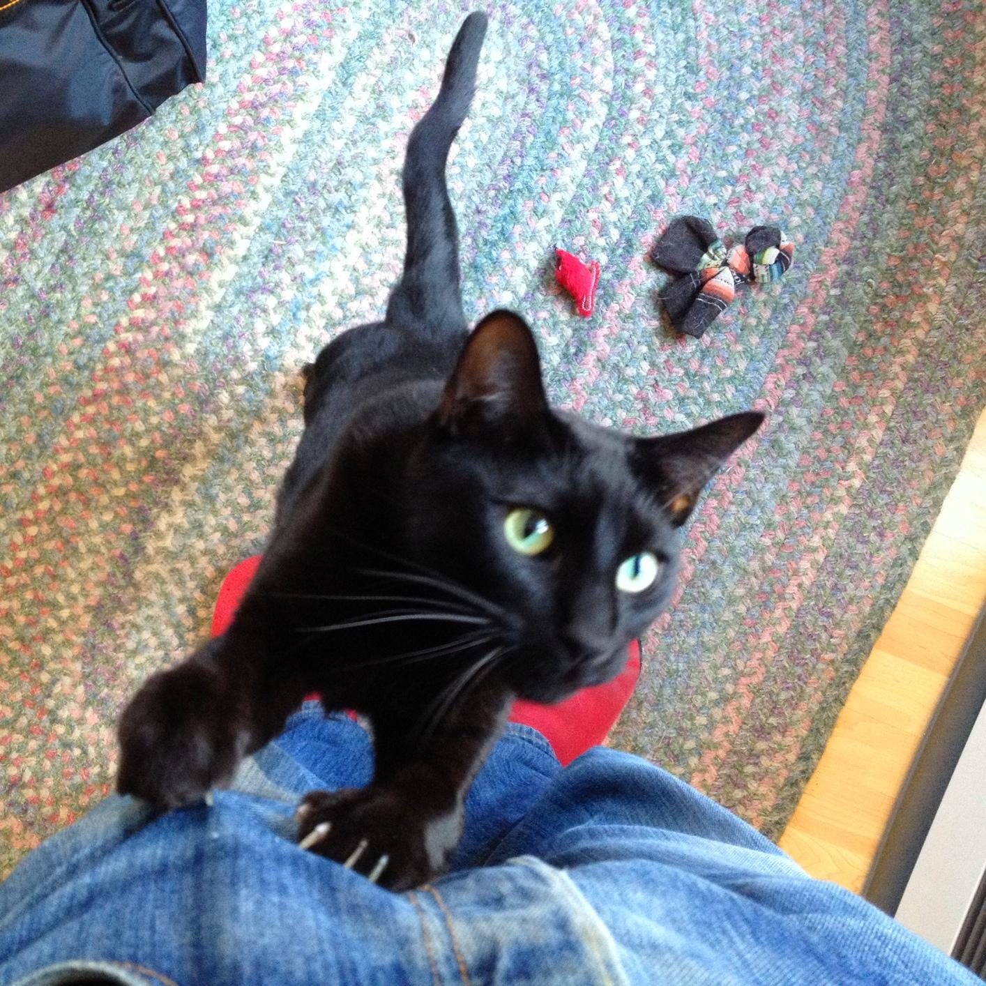
Pick me up!
Tallys died today after a short fight with an unknown disease. We got him and his two brothers from a shelter foster litter and as soon as we met him as a tiny kitten, we knew he was one of the kittens we wanted to adopt. He was the smallest kitten in the litter, was extremely friendly and very snuggly, and he remained that way for his short life. He would spend all night curled up at my feet, or under the covers with Andrea, and in the morning he’d come downstairs and ask to be picked up while I made breakfast. He loved to be up on my shoulders, purring and kneading, and occasionally scolding me if I wasn’t petting him enough. He played with my feet under the covers, and would bring cat toys downstairs during the day while we were at work and the dogs were outside. He also made friends with all the dogs, and especially Monte, who would come in the house and bark until his friend Tallys came down to nuzzle him and play.
He also loved heat, so he was always the cat baking himself in the direct sun in the window, and especially liked winter because of the heat the wood stove put out. He’d lay in front of it (or sometimes directly under it) and his fur would get hot enough it seemed like he should be melting. And when the wood stove wasn’t cranking he’d flop down in front of our Toyo and soak up as much heat as he could.
He is survived by his brothers, Jenson and Caslon, and his two sisters living in another home in Fairbanks. Tallys, Jenson, and Caslon all got along at our house, sleeping in a ball on the bed, or chasing each other around. Tallys and Caslon would often sit opposite each other and lazily swat at each other until someone got in a good punch and they’d go bolting after each other.
He was a super sweet little cat, and our time with him was too short, but in those years he was a constant bright spot in our lives. We will miss him.
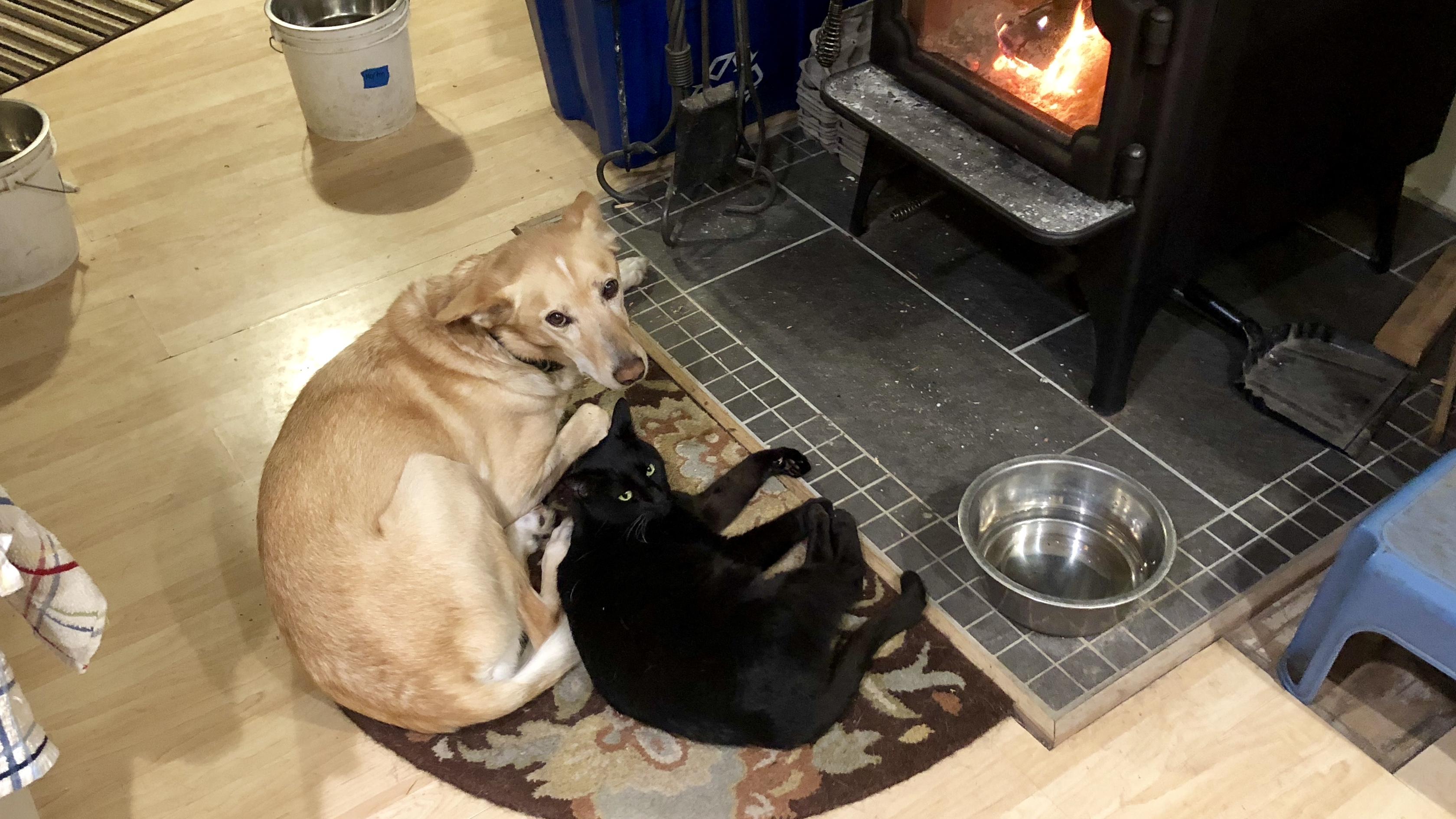
Monte and Tallys enjoying the wood stove
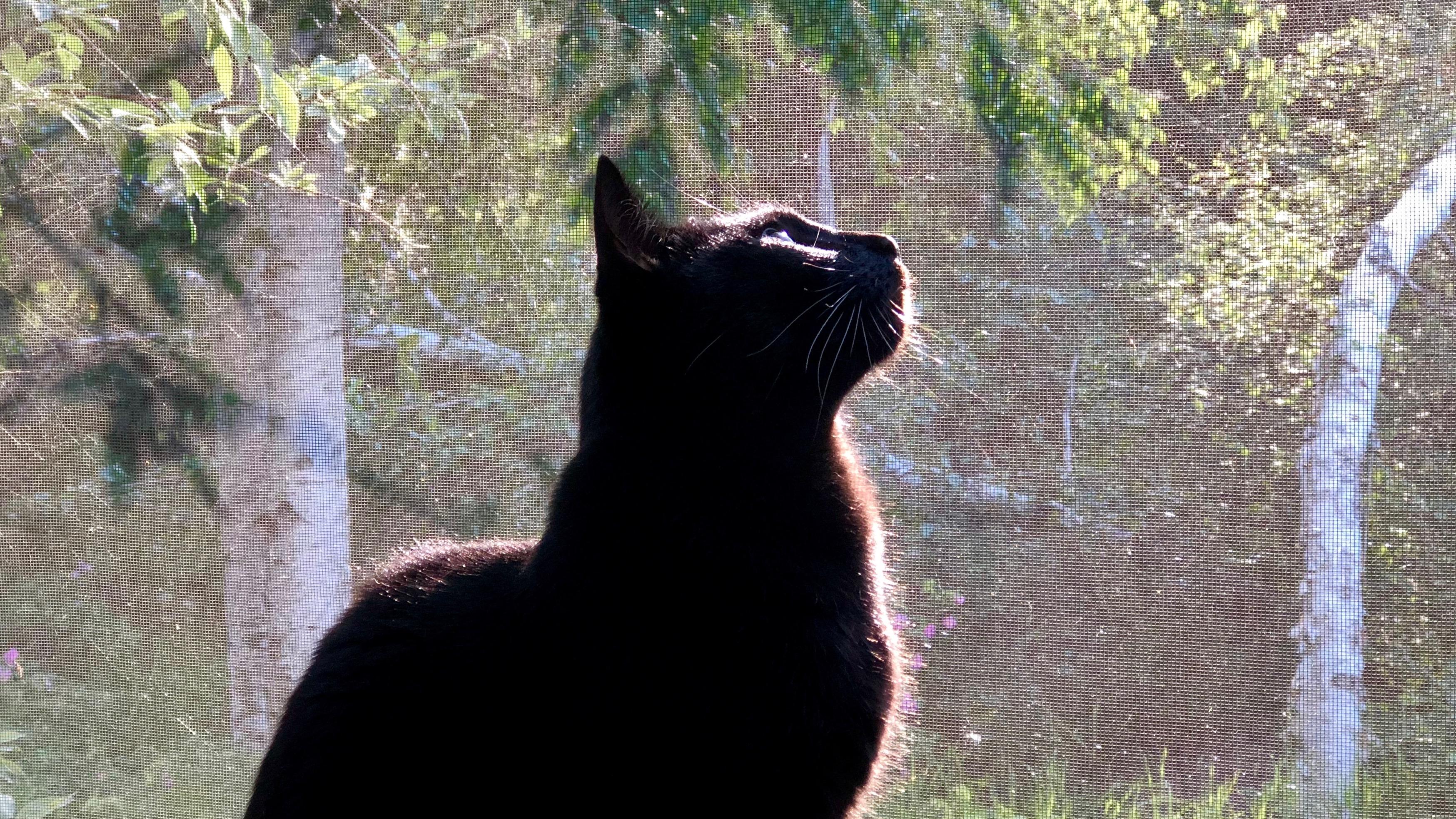
Tallys bug hunting
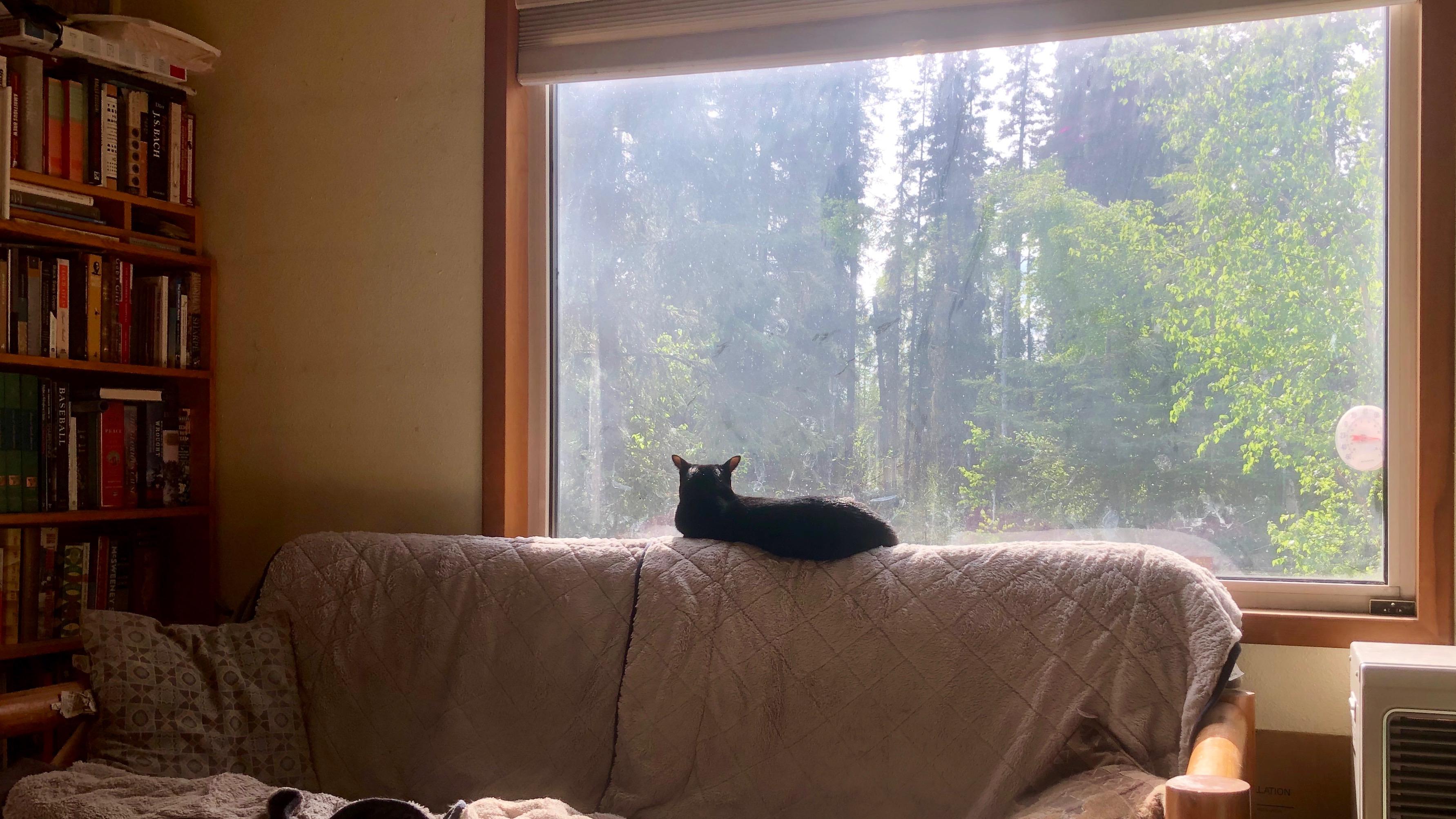
Tallys looking out the window