St. Roy
Before I went to California I decided I was finally ready to become a cell phone user with Apple’s iPhone. The contract (two years) is ridiculously long, AT&T doesn’t have the best record when it comes to service and upgrades (we don’t have 3G here in Fairbanks yet…), and I’m uncomfortable with how tight Apple is with their software and hardware. But a cell phone with a fast processor, lots of storage, built-in GPS, compass, motion sensors and a camera that can shoot stills and video? Plus a wide range of apps and an SDK to allow me to develop my own? I couldn’t resist. After verifying we could get service at our house (typically two, weak bars), we signed up and I picked up my phone at the Apple store in San Francisco on my way to Berkeley. Andrea got hers a few days later here in Fairbanks.
The iPhone is everything I thought it would be. The hardware and most of the software is incredible, and it’s already changing (improving, thus far) the way I live my life. The closed nature of it still bothers me, but I’m willing to give it a chance before I consider jailbreaking it.
What does this have to do with The Woodwright’s Shop and St. Roy? Well, one of the apps I have on my iPhone is called What’s On, and as I was perusing the TV schedule to see what baseball game was on FOX (what a surprise: Red Sox vs. Yankees) I noticed that The Woodwright’s Shop had a little HD icon next to it. Sure enough, when I flipped it on, there was St. Roy boring star-shaped holes into walnut in full high-definition video!
Sweet!

Preserves
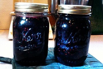
After a week and a half in Berkeley and a quick trip to Anchorage for work, I finally feel like things are getting back to normal. Last weekend we bought a bunch of stuff at the Farmer’s Market, including a small basket of raspberries. I had planned to make some raspberry bars, but when I looked at them today, they seemed a bit soft for something like that. On Sunday we picked a half gallon of blueberries from the power line, so making preserves from the combination seemed like a good idea. Here’s the recipe I used:
Ingredients:
- 1 small basket fresh raspberries (approximately 2 cups)
- Same weight of fresh blueberries (~2 cups)
- 1 apple, peeled, cored, and chopped small
- Juice from ½ lemon
- 1 T water
- 3 cups sugar
Cooking:
- Bring fruit and liquids to a boil.
- Boil 5 minutes to soften apples.
- Add sugar and mix.
- Purée in food processor.
- Return to boil.
- Boil 10–15 minutes until the pectin is ready (it gels on the back of a spoon as it cools)
Canning:
- Pour or ladle into hot canning jars (2 pint jars for this quantity), boil in hot water bath for 10 minutes.
I’m not sure if the apple is necessary, but the recipe I was looking at included pectin and I didn’t have any. The Interwebs informed me that apples contain a lot of pectin, so I threw that in the pot as well. The food processor step was included because I wasn’t convinced the apples would get mushed up enough to disappear in the mix.
Yesterday I looked at how wind might be affecting my bicycling to and from work. Today I’ll examine the idea that Miller Hill is confounding the effect of wind on average speed by excluding this portion of the trip from the analysis. To do this, I include a bounding box comparison in the SQL statement that extracts the wind factors for track points. The additional WHERE condition looks like this:
ST_Within(point_utm, ST_SetSRID(ST_MakeBox2D(ST_Point(454861,7193973), ST_Point(458232,7199159)), 32606))
The same ST_Within test is used in the calculation of average speed for each of the trips from work to home. After compiling the wind factors and average speeds, we compare the two using R. Here are the updated results:
lm(formula = mph ~ wind, data = data)

Residuals:
     Min       1Q   Median       3Q      Max
-1.87808 -0.55299  0.04038  0.62790  1.19076

Coefficients:
            Estimate Std. Error t value Pr(>|t|)
(Intercept)  16.8544     0.2176  77.442   <2e-16 ***
wind          0.3896     0.2002   1.946   0.0683 .
---
Signif. codes:  0 ‘***’ 0.001 ‘**’ 0.01 ‘*’ 0.05 ‘.’ 0.1 ‘ ’ 1

Residual standard error: 0.9445 on 17 degrees of freedom
Multiple R-squared: 0.1822,     Adjusted R-squared: 0.1341
F-statistic: 3.788 on 1 and 17 DF,  p-value: 0.06834
This time around the model and both coefficients are statistically significant (finally!), and “wind factor” is positively correlated with my average speed over the part of the route that doesn’t include Miller Hill and Railroad drive. It’s not a major contributor, but it does explain approximately 18% of the variation in average speed.
I decided to look at wind a little more deeply after yesterday’s bike ride home. It seemed clear to me that the wind was strongly at my back for much of the route. It wasn’t my fastest ride home, but it was close, and it didn’t feel like I was working all that hard.
Here’s the process. First, examine all my bicycling tracks individually, using PostGIS’s ST_Azimuth function to calculate the direction I was traveling at each point. The query uses another of the new window functions (lead) in PostgreSQL 8.4.
SELECT
    point_id, dt_local,
    ST_Azimuth(
        point_utm,
        lead(point_utm) OVER (PARTITION BY tid ORDER BY dt_local)
    ) / (2 * pi()) *360
FROM points
WHERE tid = TID
ORDER BY dt_local;
Then, for each point, find the direction the wind was blowing. This is a pretty slow query, but I haven’t found a better way to compare timestamps in the database to find the closest record. This technique, based on converting both timestamps to “epoch,” which is the number of seconds since January 1st, 1970, is faster than using an interval type of operation (like: WHERE obs_dt - POINT_DT BETWEEN interval '-3 minutes' AND interval '3 minutes').
SELECT obs_dt, wdir, wspd
FROM observations
WHERE abs(extract(epoch from obs_dt) - extract(epoch from POINT_DT)) < 5 * 60
    AND wspd IS NOT NULL
    AND wdir IS NOT NULL
ORDER BY abs(extract(epoch from obs_dt) - extract(epoch from POINT_DT))
LIMIT 1;
Now I’ve got the direction I was traveling and the direction the wind is coming from. I wrote a Python function that returns a value from –1 (wind is in my face) to 1 (wind is at my back). The procedure is to convert the wind directions to unit u and v vectors and get the distance between the endpoints of each vector. The distances are then scaled such that wind behind the direction traveled range from 0 – 1, and from –1 – 0 for wind blowing against the direction traveled.
def wind_effect(mydir, winddir):
    """ Returns a number from 1 (wind at my back) to -1 (wind in my face)
        based on the directions passed in.

        Remember that wind direction is where the wind is *from*, so a
        wind direction of 0 and a mydir of 0 means the wind is in my face.
    """
    try:
        mydir = float(mydir)
        winddir = float(winddir)
    except:
        return(None)

    my_spd = 1.0
    wind_spd = 1.0
    u_mydir = -1 * my_spd * math.sin(math.radians(mydir))
    v_mydir = -1 * my_spd * math.cos(math.radians(mydir))
    u_winddir = -1 * wind_spd * math.sin(math.radians(winddir))
    v_winddir = -1 * wind_spd * math.cos(math.radians(winddir))
    distance = math.sqrt((u_mydir - u_winddir)**2 + (v_mydir - v_winddir)**2)
    factor = (1.41421356 - distance)
    if factor < 0.0:
        factor = factor / -0.58578644
    else:
        factor = factor / -1.41421356

    return(factor)
Finally, multiply this value by the wind speed at that time, and sum all these values for an entire bicycling track. The result is a “wind factor.” A positive wind factor means the wind was generally at my back during the ride, negative means it was blowing in my face. Yesterday’s ride home had the highest wind factor (1.07) among trips since June. So the wind really was at my back!
Can “wind factor” help predict average speed? Here’s the R and results:
$ R --save < wind_from_abr.R
> data<-read.table('wind_factor_from_abr',header=TRUE)
> model<-lm(speed ~ wind, data)
> summary(model)

Call:
lm(formula = speed ~ wind, data = data)

Residuals:
     Min       1Q   Median       3Q      Max
-0.90395 -0.46782 -0.04334  0.40286  0.85918

Coefficients:
            Estimate Std. Error t value Pr(>|t|)
(Intercept)  14.7796     0.1471  100.48   <2e-16 ***
wind          0.4369     0.2875    1.52    0.147
---
Signif. codes:  0 ‘***’ 0.001 ‘**’ 0.01 ‘*’ 0.05 ‘.’ 0.1 ‘ ’ 1

Residual standard error: 0.5522 on 17 degrees of freedom
Multiple R-squared: 0.1196,     Adjusted R-squared: 0.06784
F-statistic:  2.31 on 1 and 17 DF,  p-value: 0.1469
Hmm. Not a whole lot of help here. The model is close to being statistically significant (although it’s not…), and it’s not very predictive (only 12% of the variation in average speed is explained by wind factor). However, the directionality of the (not quite statistically significant) wind coefficient is correct. A positive wind factor is (weakly) correlated with a higher average speed.
Thinking more about my route from work, I suspect that the route is actually two trips: the trip from ABR to the bottom of Miller Hill (4.8 miles) and the two mile trip over Miller Hill to our house. I’ll bet that wind becomes statistically significant if I only consider the first part of the trip: wind doesn’t have as much effect on a hill climb, and after making it over the top, the rest is a bumpy, gravel road where speed is determined more by safety than wind or how hard I’m pedalling. I think this might also resolve the question of why the ride home is so much easier than to work. It’s not because I’m glad to be out of work or because I’m carrying a lunchbox full of food to work, it’s because it’s downhill from ABR to the bottom of Miller Hill.
It’s interesting riding the same route back and forth to work every day. I have a perception that the wind is always in my face, and wondered if maybe the wind tends to be going one direction in the morning, and another in the afternoon when I’m riding home. Despite the fact that riding home seems much easier than riding to work, the wind always seems stronger.
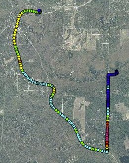
If you look at the little map of my bicycling route from work on the right, you can see that the major portion of the trip is in a northwesterly (to work) or southeasterly (from work) direction. The long stretch that’s north/south is Miller Hill, and wind doesn’t really matter on that section of the route because it’s a steep hill. The color of the dots indicate speed from blue (slow) to red (fast).
I took a look at the wind data from our weather station for the days I bicycled to work; for the two hours before and after each ride on those dates. The weather database has a binned summary of wind direction (each row in the table shows the number of five-minute observations where the wind was blowing in a particular cardinal direction) and an average speed. I multiplied the two for each hour during my rides, and then summed them over all my rides this year. The plot below shows what the data looks like.
And, for reference, the SQL query, data set and gnuplot script. It took me forever to figure out how to make gnuplot make a histogram of this data.
Wind direction, to and from work
I was right about it being windier on my ride home from work. But, my perception that the wind is always in my face isn’t right. In both the morning and afternoon, there are two predominant wind directions, northwest (which would be at my back on the way home) and south-southeast (in my face). This is one of those cases where I notice when the wind is in my face, but when it’s at my back it doesn’t register.
At some point I’ll have to see if there’s any relationship between my average speed and the wind. At least then I’d have something to blame when I arrive at my destination with a slow time.

