Introduction
For the past two years I’ve played Yahoo fantasy baseball with a group of friends. It’s a fun addition to watching games because it requires you to pay attention to more than just the players on the teams you root for (especially important if your favorite “team” is the Athletics).
Last year we had a draft party and it was interesting to see how different people approached the draft. Some of us chose players for emotional reasons like whether they played for the team they rooted for or what country the player was from, and some used a very analytical approach. The last two years I’ve tended to be more on the emotional side, choosing preferrentialy for former Oakland Athletcs players in the first year, and current Phillies last year. Some brought computers to track choices and rankings, and some didn’t bring anything at all except their phones and minds.
I’ve been working on my draft strategy for next year, and plan to use a more analytical approach to the draft. I’m working on an app that will have all the players in draft ranked, and allow me to easily mark off who has been selected, and who I’ve added to my team in real time as the draft is underway.
One of the important considerations for choosing any player is what positions they can play. Not only do you need to field a complete team with pitchers, catchers, infielders, and outfielders, but some players are capable of playing multiple positions, and those players can be more valuable to a fantasy manager than their pure numbers would suggest because you can plug them into different positions on any given day. Last year I had Alec Bohm on my team, which allowed me to fill either first base (typically manned by Vladimir Gurerro Jr) or third, depending on what teams were playing or who might be injured or getting a day off. I used Brandon Drury to great effect two years ago because he was eligible for three infield positions.
Positional eligibility for Yahoo fantasy follows these rules:
- Position eligibility – 5 starts or 10 total appearances in a position.
- Pitcher eligibility – 3 starts to be a starter, or 5 relief appearances to qualify as a reliever.
In this post I will use Retrosheet event data to determine the positional eligibility for all the players who played in the majors last year. In cases where a player in the draft hasn’t played in the majors but is likely to reach Major League Baseball in 2024, I’ll just use whatever position the projections have him in.
Methods
I’m going to use the retrosheet R package to load the event files for 2023, then determine how many games each player started and substituted at each position, and apply Yahoo’s rules to determine eligibility.
We’ll load some libraries, get the team IDs, and map Retrosheet position IDs to the usual position abbreviations.
library(tidyr)
library(dplyr)
library(purrr)
library(retrosheet)
library(glue)

YEAR <- 2023

team_ids <- getTeamIDs(YEAR)

positions <- tribble(
   ~fieldPos, ~pos,
   "1", "P",
   "2", "C",
   "3", "1B",
   "4", "2B",
   "5", "3B",
   "6", "SS",
   "7", "LF",
   "8", "CF",
   "9", "RF",
   "10", "DH",
   "11", "PH",
   "12", "PR"
)
Next, we write a function to retrieve the data for a single team’s home games, and extract the starting and subtitution information, which are stored as $start and $sub matrices in the Retrosheet event files. Then loop over this function for every team, and convert position ID to the position abbreviations.
get_pbp <- function(team_id) {
   print(glue("loading {team_id}"))

   pbp <- getRetrosheet("play", YEAR, team_id)

   starters <- map(
      seq(1, length(pbp)),
      function(game) {
      pbp[[game]]$start |>
         as_tibble()
      }
   ) |>
      list_rbind() |>
      mutate(start_sub = "start")

   subs <- map(
      seq(1, length(pbp)),
      function(game) {
      pbp[[game]]$sub |>
         as_tibble()
      }
   ) |>
      list_rbind() |>
      mutate(start_sub = "sub")

   bind_rows(starters, subs)
}

pbp_start_sub <- map(
   team_ids,
   get_pbp
) |>
   list_rbind() |>
   inner_join(positions, by = "fieldPos")
That data frame looks like this, with one row for every player that played in any game during the 2023 regular season:
# A tibble: 76,043 × 7
   retroID  name                  team  batPos fieldPos start_sub pos
   <chr>    <chr>                 <chr> <chr>  <chr>    <chr>     <chr>
   1 sprig001 George Springer       0     1      9        start     RF
   2 bichb001 Bo Bichette           0     2      6        start     SS
   3 guerv002 Vladimir Guerrero Jr. 0     3      3        start     1B
   4 chapm001 Matt Chapman          0     4      5        start     3B
   5 merrw001 Whit Merrifield       0     5      7        start     LF
   6 kirka001 Alejandro Kirk        0     6      2        start     C
   7 espis001 Santiago Espinal      0     7      4        start     2B
   8 luplj001 Jordan Luplow         0     8      10       start     DH
   9 kierk001 Kevin Kiermaier       0     9      8        start     CF
  10 bassc001 Chris Bassitt         0     0      1        start     P
# ℹ 76,033 more rows
Next, we convert that into appearances by grouping the data by player, whether they were a starter or substitute, and by their position. Since each row in the original data frame is per game, we can use n() to count the games each player started and subbed for each position.
appearances <- pbp_start_sub |>
   group_by(retroID, name, start_sub, pos) |>
   summarize(games = n(), .groups = "drop") |>
   pivot_wider(names_from = start_sub, values_from = games)
That looks like this:
# A tibble: 3,479 × 5
   retroID  name          pos     sub start
   <chr>    <chr>         <chr> <int> <int>
   1 abadf001 Fernando Abad P         6    NA
   2 abboa001 Andrew Abbott P        NA    21
   3 abboc001 Cory Abbott   P        22    NA
   4 abrac001 CJ Abrams     SS        3   148
   5 abrac001 CJ Abrams     PH        2    NA
   6 abrac001 CJ Abrams     PR        1    NA
   7 abrea001 Albert Abreu  P        45    NA
   8 abreb002 Bryan Abreu   P        72    NA
   9 abrej003 Jose Abreu    1B       NA   134
  10 abrej003 Jose Abreu    DH       NA     7
# ℹ 3,469 more rows
Finally, we group by the player and position, calculate eligibility, then group by player and combine all the positions they are eligible for into a single string. There’s a little funny business at the end to remove pitching eligibility from position players who are called into action as pitchers in blow out games, and player suffixes, which may or may not be necessary for matching against your projection ranks.
eligibility <- appearances |>
   filter(pos != "PH", pos != "PR") |>
   mutate(
      sub = if_else(is.na(sub), 0, sub),
      start = if_else(is.na(start), 0, start),
      total = sub + start,
      eligible = case_when(
      pos == "P" & start >= 3 & sub >= 5 ~ "SP,RP",
      pos == "P" & start >= 3 ~ "SP",
      pos == "P" & sub >= 5 ~ "RP",
      pos == "P" ~ "P",
      start >= 5 | total >= 10 ~ pos,
      TRUE ~ NA
      )
   ) |>
   filter(!is.na(eligible)) |>
   arrange(retroID, name, desc(total)) |>
   group_by(retroID, name) |>
   summarize(
      eligible = paste(eligible, collapse = ","),
      eligible = gsub(",P$", "", eligible),
      .groups = "drop"
   ) |>
   mutate(
      name = gsub(" (Jr.|II|IV)", "", name)
   )
Here’s a look at the final results. You can download the full data as a CSV file below.
# A tibble: 1,402 × 3
   retroID  name            eligible
   <chr>    <chr>           <chr>
   1 abadf001 Fernando Abad   RP
   2 abboa001 Andrew Abbott   SP
   3 abboc001 Cory Abbott     RP
   4 abrac001 CJ Abrams       SS
   5 abrea001 Albert Abreu    RP
   6 abreb002 Bryan Abreu     RP
   7 abrej003 Jose Abreu      1B,DH
   8 abrew002 Wilyer Abreu    CF,LF
   9 acevd001 Domingo Acevedo RP
  10 actog001 Garrett Acton   RP
# ℹ 1,392 more rows
Who is eligible for the most positions? Here's the top 20:
   retroID  name              eligible
   <chr>    <chr>             <chr>
 1 herne001 Enrique Hernandez SS,2B,CF,3B,LF,1B
 2 diaza003 Aledmys Diaz      3B,SS,LF,2B,1B,DH
 3 hampg001 Garrett Hampson   SS,CF,RF,2B,LF
 4 mckiz001 Zach McKinstry    3B,2B,RF,LF,SS
 5 ariag002 Gabriel Arias     SS,1B,RF,3B
 6 bertj001 Jon Berti         SS,3B,LF,2B
 7 biggc002 Cavan Biggio      2B,RF,1B,3B
 8 cabro002 Oswaldo Cabrera   LF,RF,3B,SS
 9 castw003 Willi Castro      LF,CF,3B,2B
10 dubom001 Mauricio Dubon    2B,CF,LF,SS
11 edmat001 Tommy Edman       2B,SS,CF,RF
12 gallj002 Joey Gallo        1B,LF,CF,RF
13 ibana001 Andy Ibanez       2B,3B,LF,RF
14 newmk001 Kevin Newman      3B,SS,2B,1B,DH
15 rengl001 Luis Rengifo      2B,SS,3B,RF
16 senzn001 Nick Senzel       3B,LF,CF,RF
17 shorz001 Zack Short        2B,SS,3B,RP
18 stees001 Spencer Steer     1B,3B,LF,2B,DH
19 vargi001 Ildemaro Vargas   3B,2B,SS,LF
20 vierm001 Matt Vierling     RF,LF,3B,CF
References and Acknowledgements
The information used here was obtained free of charge from and is copyrighted by Retrosheet. Interested parties may contact Retrosheet at “www.retrosheet.org”.
Introduction
Often when I’m watching Major League Baseball games a player will come up to bat or pitch and I’ll comment “former Oakland Athletic” and the player’s name. It seems like there’s always one or two players on the roster of every team that used to be an Athletic.
Let’s find out. We’ll use the Retrosheet database again, this time using the roster lists from 1990 through 2014 and comparing it against the 40-man rosters of current teams. That data will have to be scraped off the web, since Retrosheet data doesn’t exist for the current season and rosters change frequently during the season.
Methods
As usual, I’ll use R for the analysis, and rmarkdown to produce this post.
library(plyr)
library(dplyr)
library(rvest)
options(stringsAsFactors=FALSE)
We’re using plyr and dplyr for most of the data manipulation and rvest to grab the 40-man rosters for each team from the MLB website. Setting stringsAsFactors to false prevents various base R packages from converting everything to factors. We're not doing any statistics with this data, so factors aren't necessary and make comparisons and joins between data frames more difficult.
Players by team for previous years
Load the roster data:
retrosheet_db <- src_postgres(host="localhost", port=5438,
                              dbname="retrosheet", user="cswingley")

rosters <- tbl(retrosheet_db, "rosters")

all_recent_players <-
     rosters %>%
     filter(year>1989) %>%
     collect() %>%
     mutate(player=paste(first_name, last_name),
            team=team_id) %>%
     select(player, team, year)

save(all_recent_players, file="all_recent_players.rdata", compress="gzip")
The Retrosheet database lives in PostgreSQL on my computer, but one of the advantages of using dplyr for retrieval is it would be easy to change the source statement to connect to another sort of database (SQLite, MySQL, etc.) and the rest of the commands would be the same.
We only grab data since 1990 and we combine the first and last names into a single field because that’s how player names are listed on the 40-man roster pages on the web.
Now we filter the list down to Oakland Athletic players, combine the rows for each Oakland player, summarizing the years they played for the A’s into a single column.
oakland_players <- all_recent_players %>%
    filter(team=='OAK') %>%
    group_by(player) %>%
    summarise(years=paste(year, collapse=', '))
Here’s what that looks like:
kable(head(oakland_players))
| player | years |
|---|---|
| A.J. Griffin | 2012, 2013 |
| A.J. Hinch | 1998, 1999, 2000 |
| Aaron Cunningham | 2008, 2009 |
| Aaron Harang | 2002, 2003 |
| Aaron Small | 1996, 1997, 1998 |
| Adam Dunn | 2014 |
| ... | ... |
Current 40-man rosters
Major League Baseball has the 40-man rosters for each team on their site. In order to extract them, we create a list of the team identifiers (oak, sf, etc.), then loop over this list, grabbing the team name and all the player names. We also set up lists for the team names (“Athletics”, “Giants”, etc.) so we can replace the short identifiers with real names later.
teams=c("ana", "ari", "atl", "bal", "bos", "cws", "chc", "cin", "cle", "col",
        "det", "mia", "hou", "kc", "la", "mil", "min", "nyy", "nym", "oak",
        "phi", "pit", "sd", "sea", "sf", "stl", "tb", "tex", "tor", "was")

team_names = c("Angels", "Diamondbacks", "Braves", "Orioles", "Red Sox",
               "White Sox", "Cubs", "Reds", "Indians", "Rockies", "Tigers",
               "Marlins", "Astros", "Royals", "Dodgers", "Brewers", "Twins",
               "Yankees", "Mets", "Athletics", "Phillies", "Pirates",
               "Padres", "Mariners", "Giants", "Cardinals", "Rays", "Rangers",
               "Blue Jays", "Nationals")

get_players <- function(team) {
    # reads the 40-man roster data for a team, returns a data frame

    roster_html <- html(paste("http://www.mlb.com/team/roster_40man.jsp?c_id=",
                              team,
                              sep=''))

    players <- roster_html %>%
        html_nodes("#roster_40_man a") %>%
        html_text()

    data.frame(team=team, player=players)
}

current_rosters <- ldply(teams, get_players)

save(current_rosters, file="current_rosters.rdata", compress="gzip")
Here’s what that data looks like:
kable(head(current_rosters))
| team | player |
|---|---|
| ana | Jose Alvarez |
| ana | Cam Bedrosian |
| ana | Andrew Heaney |
| ana | Jeremy McBryde |
| ana | Mike Morin |
| ana | Vinnie Pestano |
| ... | ... |
Combine the data
To find out how many players on each Major League team used to play for the A’s we combine the former A’s players with the current rosters using player name. This may not be perfect due to differences in spelling (accented characters being the most likely issue), but the results look pretty good.
roster_with_oakland_time <- current_rosters %>%
    left_join(oakland_players, by="player") %>%
    filter(!is.na(years))

kable(head(roster_with_oakland_time))
| team | player | years |
|---|---|---|
| ana | Huston Street | 2005, 2006, 2007, 2008 |
| ana | Grant Green | 2013 |
| ana | Collin Cowgill | 2012 |
| ari | Brad Ziegler | 2008, 2009, 2010, 2011 |
| ari | Cliff Pennington | 2008, 2009, 2010, 2011, 2012 |
| atl | Trevor Cahill | 2009, 2010, 2011 |
| ... | ... | ... |
You can see from this table (just the first six rows of the results) that the Angels have three players that were Athletics.
Let’s do the math and find out how many former A’s are on each team’s roster.
n_former_players_by_team <-
    roster_with_oakland_time %>%
        group_by(team) %>%
        arrange(player) %>%
        summarise(number_of_players=n(),
                  players=paste(player, collapse=", ")) %>%
        arrange(desc(number_of_players)) %>%
        inner_join(data.frame(team=teams, team_name=team_names),
                   by="team") %>%
        select(team_name, number_of_players, players)

names(n_former_players_by_team) <- c('Team', 'Number',
                                     'Former Oakland Athletics')
kable(n_former_players_by_team,
      align=c('l', 'r', 'r'))
| Team | Number | Former Oakland Athletics |
|---|---|---|
| Athletics | 22 | A.J. Griffin, Andy Parrino, Billy Burns, Coco Crisp, Craig Gentry, Dan Otero, Drew Pomeranz, Eric O'Flaherty, Eric Sogard, Evan Scribner, Fernando Abad, Fernando Rodriguez, Jarrod Parker, Jesse Chavez, Josh Reddick, Nate Freiman, Ryan Cook, Sam Fuld, Scott Kazmir, Sean Doolittle, Sonny Gray, Stephen Vogt |
| Astros | 5 | Chris Carter, Dan Straily, Jed Lowrie, Luke Gregerson, Pat Neshek |
| Braves | 4 | Jim Johnson, Jonny Gomes, Josh Outman, Trevor Cahill |
| Rangers | 4 | Adam Rosales, Colby Lewis, Kyle Blanks, Michael Choice |
| Angels | 3 | Collin Cowgill, Grant Green, Huston Street |
| Cubs | 3 | Chris Denorfia, Jason Hammel, Jon Lester |
| Dodgers | 3 | Alberto Callaspo, Brandon McCarthy, Brett Anderson |
| Mets | 3 | Anthony Recker, Bartolo Colon, Jerry Blevins |
| Yankees | 3 | Chris Young, Gregorio Petit, Stephen Drew |
| Rays | 3 | David DeJesus, Erasmo Ramirez, John Jaso |
| Diamondbacks | 2 | Brad Ziegler, Cliff Pennington |
| Indians | 2 | Brandon Moss, Nick Swisher |
| White Sox | 2 | Geovany Soto, Jeff Samardzija |
| Tigers | 2 | Rajai Davis, Yoenis Cespedes |
| Royals | 2 | Chris Young, Joe Blanton |
| Marlins | 2 | Dan Haren, Vin Mazzaro |
| Padres | 2 | Derek Norris, Tyson Ross |
| Giants | 2 | Santiago Casilla, Tim Hudson |
| Nationals | 2 | Gio Gonzalez, Michael Taylor |
| Red Sox | 1 | Craig Breslow |
| Rockies | 1 | Carlos Gonzalez |
| Brewers | 1 | Shane Peterson |
| Twins | 1 | Kurt Suzuki |
| Phillies | 1 | Aaron Harang |
| Mariners | 1 | Seth Smith |
| Cardinals | 1 | Matt Holliday |
| Blue Jays | 1 | Josh Donaldson |
Pretty cool. I do notice one problem: there are actually two Chris Young’s playing in baseball today. Chris Young the outfielder played for the A’s in 2013 and now plays for the Yankees. There’s also a pitcher named Chris Young who shows up on our list as a former A’s player who now plays for the Royals. This Chris Young never actually played for the A’s. The Retrosheet roster data includes which hand (left and/or right) a player bats and throws with, and it’s possible this could be used with the MLB 40-man roster data to eliminate incorrect joins like this, but even with that enhancement, we still have the problem that we’re joining on things that aren’t guaranteed to uniquely identify a player. That’s the nature of attempting to combine data from different sources.
One other interesting thing. I kept the A’s in the list because the number of former A’s currently playing for the A’s is a measure of how much turnover there is within an organization. Of the 40 players on the current A’s roster, only 22 of them have ever played for the A’s. That means that 18 came from other teams or are promotions from the minors that haven’t played for any Major League teams yet.
All teams
Teams with players on other teams
Now that we’ve looked at how many A’s players have played for other teams, let’s see how the number of players playing for other teams is related to team. My gut feeling is that the A’s will be at the top of this list as a small market, low budget team who is forced to turn players over regularly in order to try and stay competitive.
We already have the data for this, but need to manipulate it in a different way to get the result.
teams <- c("ANA", "ARI", "ATL", "BAL", "BOS", "CAL", "CHA", "CHN", "CIN",
           "CLE", "COL", "DET", "FLO", "HOU", "KCA", "LAN", "MIA", "MIL",
           "MIN", "MON", "NYA", "NYN", "OAK", "PHI", "PIT", "SDN", "SEA",
           "SFN", "SLN", "TBA", "TEX", "TOR", "WAS")

team_names <- c("Angels", "Diamondbacks", "Braves", "Orioles", "Red Sox",
                "Angels", "White Sox", "Cubs", "Reds", "Indians", "Rockies",
                "Tigers", "Marlins", "Astros", "Royals", "Dodgers", "Marlins",
                "Brewers", "Twins", "Expos", "Yankees", "Mets", "Athletics",
                "Phillies", "Pirates", "Padres", "Mariners", "Giants",
                "Cardinals", "Rays", "Rangers", "Blue Jays", "Nationals")

players_on_other_teams <- all_recent_players %>%
    group_by(player, team) %>%
    summarise(years=paste(year, collapse=", ")) %>%
    inner_join(current_rosters, by="player") %>%
    mutate(current_team=team.y, former_team=team.x) %>%
    select(player, current_team, former_team, years) %>%
    inner_join(data.frame(former_team=teams, former_team_name=team_names),
                by="former_team") %>%
    group_by(former_team_name, current_team) %>%
    summarise(n=n()) %>%
    group_by(former_team_name) %>%
    arrange(desc(n)) %>%
    mutate(rank=row_number()) %>%
    filter(rank!=1) %>%
    summarise(n=sum(n)) %>%
    arrange(desc(n))
This is a pretty complicated set of operations. The main trick (and possible flaw in the analysis) is to get a list similar to the one we got for the A’s earlier, and eliminate the first row (the number of players on a team who played for that same team in the past) before counting the total players who have played for other teams. It would probably be better to eliminate that case using team name, but the team codes vary between Retrosheet and the MLB roster data.
Here are the results:
names(players_on_other_teams) <- c('Former Team', 'Number of players')

kable(players_on_other_teams)
| Former Team | Number of players |
|---|---|
| Athletics | 57 |
| Padres | 57 |
| Marlins | 56 |
| Rangers | 55 |
| Diamondbacks | 51 |
| Braves | 50 |
| Yankees | 50 |
| Angels | 49 |
| Red Sox | 47 |
| Pirates | 46 |
| Royals | 44 |
| Dodgers | 43 |
| Mariners | 42 |
| Rockies | 42 |
| Cubs | 40 |
| Tigers | 40 |
| Astros | 38 |
| Blue Jays | 38 |
| Rays | 38 |
| White Sox | 38 |
| Indians | 35 |
| Mets | 35 |
| Twins | 33 |
| Cardinals | 31 |
| Nationals | 31 |
| Orioles | 31 |
| Reds | 28 |
| Brewers | 26 |
| Phillies | 25 |
| Giants | 24 |
| Expos | 4 |
The A’s are indeed on the top of the list, but surprisingly, the Padres are also at the top. I had no idea the Padres had so much turnover. At the bottom of the list are teams like the Giants and Phillies that have been on recent winning streaks and aren’t trading their players to other teams.
Current players on the same team
We can look at the reverse situation: how many players on the current roster played for that same team in past years. Instead of removing the current × former team combination with the highest number, we include only that combination, which is almost certainly the combination where the former and current team is the same.
players_on_same_team <- all_recent_players %>%
    group_by(player, team) %>%
    summarise(years=paste(year, collapse=", ")) %>%
    inner_join(current_rosters, by="player") %>%
    mutate(current_team=team.y, former_team=team.x) %>%
    select(player, current_team, former_team, years) %>%
    inner_join(data.frame(former_team=teams, former_team_name=team_names),
                by="former_team") %>%
    group_by(former_team_name, current_team) %>%
    summarise(n=n()) %>%
    group_by(former_team_name) %>%
    arrange(desc(n)) %>%
    mutate(rank=row_number()) %>%
    filter(rank==1,
           former_team_name!="Expos") %>%
    summarise(n=sum(n)) %>%
    arrange(desc(n))

names(players_on_same_team) <- c('Team', 'Number of players')

kable(players_on_same_team)
| Team | Number of players |
|---|---|
| Rangers | 31 |
| Rockies | 31 |
| Twins | 30 |
| Giants | 29 |
| Indians | 29 |
| Cardinals | 28 |
| Mets | 28 |
| Orioles | 28 |
| Tigers | 28 |
| Brewers | 27 |
| Diamondbacks | 27 |
| Mariners | 27 |
| Phillies | 27 |
| Reds | 26 |
| Royals | 26 |
| Angels | 25 |
| Astros | 25 |
| Cubs | 25 |
| Nationals | 25 |
| Pirates | 25 |
| Rays | 25 |
| Red Sox | 24 |
| Blue Jays | 23 |
| Athletics | 22 |
| Marlins | 22 |
| Padres | 22 |
| Yankees | 22 |
| Dodgers | 21 |
| White Sox | 20 |
| Braves | 13 |
The A’s are near the bottom of this list, along with other teams that have been retooling because of a lack of recent success such as the Yankees and Dodgers. You would think there would be an inverse relationship between this table and the previous one (if a lot of your former players are currently playing on other teams they’re not playing on your team), but this isn’t always the case. The White Sox, for example, only have 20 players on their roster that were Sox in the past, and there aren’t very many of them playing on other teams either. Their current roster must have been developed from their own farm system or international signings, rather than by exchanging players with other teams.
Yesterday I saw something I’ve never seen in a baseball game before: a runner getting hit by a batted ball, which according to Rule 7.08(f) means the runner is out and the ball is dead. It turns out that this isn’t as unusual an event as I’d thought (see below), but what was unusal is that this ended the game between the Angels and Giants. Even stranger, this is also how the game between the Diamondbacks and Dodgers ended.
Let’s use Retrosheet data to see how often this happens. Retrosheet data is organized into game data, roster data and event data. Event files contain a record of every event in a game and include the code BR for when a runner is hit by a batted ball. Here’s a SQL query to find all the matching events, who got hit and whether it was the last out in the game.
SELECT sub.game_id, teams, date, inn_ct, outs_ct, bat_team, event_tx,
   first_name || ' ' || last_name AS runner,
   CASE WHEN event_id = max_event_id THEN 'last out' ELSE '' END AS last_out
FROM (
   SELECT year, game_id, away_team_id || ' @ ' || home_team_id AS teams,
      date, inn_ct,
      CASE WHEN bat_home_id = 1
            THEN home_team_id
            ELSE away_team_id END AS bat_team, outs_ct, event_tx,
      CASE regexp_replace(event_tx, '.*([1-3])X[1-3H].*', E'\\1')
            WHEN '1' THEN base1_run_id
            WHEN '2' THEN base2_run_id
            WHEN '3' THEN base3_run_id END AS runner_id,
      event_id
   FROM events
   WHERE event_tx ~ 'BR'
) AS sub
   INNER JOIN rosters
      ON sub.year=rosters.year
            AND runner_id=player_id
            AND rosters.team_id = bat_team
   INNER JOIN (
      SELECT game_id, max(event_id) AS max_event_id
      FROM events
      GROUP BY game_id
   ) AS max_events
   ON sub.game_id = max_events.game_id
ORDER BY date;
Here's what the query does. The first sub-query sub finds all the events with the BR code, determines which team was batting and finds the id for the player who was running. This is joined with the roster table so we can assign a name to the runner. Finally, it’s joined with a subquery, max_events, which finds the last event in each game. Once we’ve got all that, the SELECT statement at the very top retrieves the columns of interest, and records whether the event was the last out of the game.
Retrosheet has event data going back to 1922, but the event files don’t include every game played in a season until the mid-50s. Starting in 1955 a runner being hit by a batted ball has a game twelve times, most recently in 2010. On average, runners get hit (and are called out) about fourteen times a season.
Here are the twelve times a runner got hit to end the game, since 1955. Until yesterday, when it happened twice in one day:
| Date | Teams | Batting | Event | Runner |
|---|---|---|---|---|
| 1956-09-30 | NY1 @ PHI | PHI | S4/BR.1X2(4)# | Granny Hamner |
| 1961-09-16 | PHI @ CIN | PHI | S/BR/G4.1X2(4) | Clarence Coleman |
| 1971-08-07 | SDN @ HOU | SDN | S/BR.1X2(3) | Ed Spiezio |
| 1979-04-07 | CAL @ SEA | SEA | S/BR.1X2(4) | Larry Milbourne |
| 1979-08-15 | TOR @ OAK | TOR | S/BR.3-3;2X3(4)# | Alfredo Griffin |
| 1980-09-22 | CLE @ NYA | CLE | S/BR.3XH(5) | Toby Harrah |
| 1984-04-06 | MIL @ SEA | MIL | S/BR.1X2(4) | Robin Yount |
| 1987-06-25 | ATL @ LAN | ATL | S/L3/BR.1X2(3) | Glenn Hubbard |
| 1994-06-13 | HOU @ SFN | HOU | S/BR.1X2(4) | James Mouton |
| 2001-08-04 | NYN @ ARI | ARI | S/BR.2X3(6) | David Dellucci |
| 2003-04-09 | KCA @ DET | DET | S/BR.1X2(4) | Bobby Higginson |
| 2010-06-27 | PIT @ OAK | PIT | S/BR/G.1X2(3) | Pedro Alvarez |
And all runners hit last season:
| Date | Teams | Batting | Event | Runner |
|---|---|---|---|---|
| 2014-05-07 | SEA @ OAK | OAK | S/BR/G.1X2(3) | Derek Norris |
| 2014-05-11 | MIN @ DET | DET | S/BR/G.3-3;2X3(6);1-2 | Austin Jackson |
| 2014-05-23 | CLE @ BAL | BAL | S/BR/G.2X3(6);1-2 | Chris Davis |
| 2014-05-27 | NYA @ SLN | SLN | S/BR/G.1X2(3) | Matt Holliday |
| 2014-06-14 | CHN @ PHI | CHN | S/BR/G.1X2(4) | Justin Ruggiano |
| 2014-07-13 | OAK @ SEA | SEA | S/BR/G.1X2(4) | Kyle Seager |
| 2014-07-18 | PHI @ ATL | PHI | S/BR/G.1X2(4) | Grady Sizemore |
| 2014-07-25 | BAL @ SEA | SEA | S/BR/G.1X2(4) | Brad Miller |
| 2014-08-05 | NYN @ WAS | WAS | S/BR/G.2X3(6);3-3 | Asdrubal Cabrera |
| 2014-09-04 | SLN @ MIL | SLN | S/BR/G.2X3(6);1-2 | Matt Carpenter |
| 2014-09-09 | SDN @ LAN | LAN | S/BR/G.2X3(6) | Matt Kemp |
| 2014-09-18 | BOS @ PIT | BOS | S/BR/G.3XH(5);1-2;B-1 | Jemile Weeks |
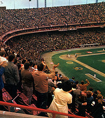
Memorial Stadium, 1971
photo by Tom Vivian
Yesterday, the Baltimore Orioles and Chicago White Sox played a game at Camden Yards in downtown Baltimore. The game was “closed to fans” due to the riots that broke out in the city after the funeral for a man who died in police custody. It’s the first time a Major League Baseball game has been played without any fans in the stands, but unfortunately it’s not the first time there have been riots in Baltimore.
After Martin Luther King, Jr. was murdered in April 1968, Baltimore rioted for six days, with local police, and more than eleven thousand National Guard, Army troops, and Marines brought in to restore order. According to wikipedia six people died, more than 700 were injured, 1,000 businesses were damaged and close to six thousand people were arrested.
At that time, the Orioles played in Memorial Stadium, about 4 miles north-northwest of where they play now. I don’t know much about that area of Baltimore, but I was curious to know whether the Orioles played any baseball games during those riots.
Retrosheet has one game, on April 10, 1968, with a reported attendance of 22,050. The Orioles defeated the Oakland Athletics by a score of 3–1. Thomas Phoebus got the win over future Hall of Famer Catfish Hunter. Other popular players in the game included Reggie Jackson, Sal Bando, Rick Mondy and Bert Campaneris for the A’s and Brooks Robinson, Frank Robinson, Davey Johnson, and Boog Powell for the Orioles.
The box score and play-by-play can be viewed here.
Next month I’ll be attending a game at Wrigley Field and my brother and I had some discussion about the best strategy for us to meet up somewhere in Chicago after the game. Knowing how long a game could be, and how many people are likely to be crowding the train platforms is useful information that can be inferred from the game data that http://www.retrosheet.org/ collects and distributes.
It’s also a good excuse to fiddle around the the IPython Notebook, pandas and the rest of the Python scientific computing stack.
I downloaded the game log data from http://www.retrosheet.org/gamelogs/index.html using this bash one-liner:
for i in `seq 1871 2012`; \
do  wget http://www.retrosheet.org/gamelogs/gl${i}.zip ; \
    unzip gl${i}.zip; \
    rm gl${i}.zip; \
done
Game Length
Game length in minutes is in column 19. Let’s read it and analyze it with Pandas.
import pandas as pd
import matplotlib.pyplot as plt
import datetime

def fix_df(input_df, cols):
    """ Pulls out the columns from cols, labels them and returns
        a new DataFrame """
    df = pd.DataFrame(index=range(len(input_df)))
    for k, v in cols.items():
        df[v] = input_df[k]

    return df

cols = {0:'dt_str', 2:'day_of_week', 3:'visiting_team',
        6:'home_team', 9:'visitor_score', 10:'home_score',
       11:'game_outs', 12:'day_night', 13:'complete',
       16:'park_id', 17:'attendance', 18:'game_time_min'}
raw_gamelogs = []
for i in range(1871, 2013):
    fn = "GL{0}.TXT".format(i)
    raw_gamelogs.append(pd.read_csv(fn, header=None, index_col=None))
raw_gamelog = pd.concat(raw_gamelogs, ignore_index=True)
gamelog = fix_df(raw_gamelog, cols)
gamelog['dte'] = gamelog.apply(
    lambda x: datetime.datetime.strptime(str(x['dt_str']), '%Y%m%d').date(),
    axis=1)
gamelog.ix[0:5, 1:] # .head() but without the dt_str col
| dow | vis | hme | vis | hme | outs | day | park | att | time | dte | |
|---|---|---|---|---|---|---|---|---|---|---|---|
| 0 | Thu | CL1 | FW1 | 0 | 2 | 54 | D | FOR01 | 200 | 120 | 1871-05-04 |
| 1 | Fri | BS1 | WS3 | 20 | 18 | 54 | D | WAS01 | 5000 | 145 | 1871-05-05 |
| 2 | Sat | CL1 | RC1 | 12 | 4 | 54 | D | RCK01 | 1000 | 140 | 1871-05-06 |
| 3 | Mon | CL1 | CH1 | 12 | 14 | 54 | D | CHI01 | 5000 | 150 | 1871-05-08 |
| 4 | Tue | BS1 | TRO | 9 | 5 | 54 | D | TRO01 | 3250 | 145 | 1871-05-09 |
| 5 | Thu | CH1 | CL1 | 18 | 10 | 48 | D | CLE01 | 2500 | 120 | 1871-05-11 |
(Note that I’ve abbreviated the column names so they fit)
The data looks reasonable, although I don’t know quite what to make of the team names from back in 1871. Now I’ll take a look at the game time data for the whole data set:
times = gamelog['game_time_min']
times.describe()
count    162259.000000
mean        153.886145
std          74.850459
min          21.000000
25%         131.000000
50%         152.000000
75%         173.000000
max       16000.000000
The statistics look reasonable, except that it’s unlikley that there was a completed game in 21 minutes, or that a game took 11 days, so we have some outliers in the data. Let’s see if something else in the data might help us filter out these records.
First the games longer than 24 hours:
print(gamelog[gamelog.game_time_min > 60 * 24][['visiting_team',
                    'home_team', 'game_outs', 'game_time_min']])
print("Removing all NaN game_outs: {0}".format(
        len(gamelog[np.isnan(gamelog.game_outs)])))
print("Max date removed: {0}".format(
        max(gamelog[np.isnan(gamelog.game_outs)].dte)))
      visiting_team home_team  game_outs  game_time_min
26664           PHA       WS1        NaN          12963
26679           PHA       WS1        NaN           4137
26685           WS1       PHA        NaN          16000
26707           NYA       PHA        NaN          15115
26716           CLE       CHA        NaN           3478
26717           DET       SLA        NaN           1800
26787           PHA       NYA        NaN           3000
26801           PHA       NYA        NaN           6000
26880           CHA       WS1        NaN           2528
26914           SLA       WS1        NaN           2245
26921           SLA       WS1        NaN           1845
26929           CLE       WS1        NaN           3215
Removing all NaN game_outs: 37890
Max date removed: 1915-10-03
There’s no value for game_outs, so there isn’t data for how long the game actually was. We remove 37,890 records by eliminating this data, but these are all games from prior to the 1916 season, so it seems reasonable:
gamelog = gamelog[pd.notnull(gamelog.game_outs)]
gamelog.game_time_min.describe()
count    156639.000000
mean        154.808975
std          32.534916
min          21.000000
25%         133.000000
50%         154.000000
75%         174.000000
max        1150.000000
What about the really short games?
gamelog[gamelog.game_time_min < 60][[
        'dte', 'game_time_min', 'game_outs']].tail()
               dte  game_time_min  game_outs
79976   1948-07-02             24         54
80138   1948-07-22             59         30
80982   1949-05-29             21         42
113455  1971-07-30             48         27
123502  1976-09-10             57         30
Many of these aren’t nine inning games because there are less than 51 outs (8 innings for a home team, 9 for the visitor in a home team win ✕ 3 innings = 51). At the moment, I’m interested in looking at how long a game is likely to be, rather than the pattern of game length over time, so we can leave these records in the data.
Now we filter the data to just the games played since 2000.
twenty_first = gamelog[gamelog['dte'] > datetime.date(1999, 12, 31)]
times_21 = twenty_first['game_time_min']
times_21.describe()
count    31580.000000
mean       175.084421
std         26.621124
min         79.000000
25%        157.000000
50%        172.000000
75%        189.000000
max        413.000000
The average game length between 2000 and 2012 is 175 minutes, or just under three hours. And three quarters of all the games played are under three hours and ten minutes.
Here’s the code to look at the distribution of these times. The top plot shows a histogram (the count of the games in each bin) and a density estimation of the same data.
The second plot is a cumulative density plot, which makes it easier to see what percentage of games are played within a certain time.
from scipy import stats
# Calculate a kernel density function
density = stats.kde.gaussian_kde(times_21)
x = range(90, 300)
rc('grid', linestyle='-', alpha=0.25)
fig, axes = plt.subplots(ncols=1, nrows=2, figsize=(8, 6))

# First plot (histogram / density)
ax = axes[0]
ax2 = ax.twinx()
h = ax.hist(times_21, bins=50, facecolor="lightgrey", histtype="stepfilled")
d = ax2.plot(x, density(x))
ax2.set_ylabel("Density")
ax.set_ylabel("Count")
plt.title("Distribution of MLB game times, 2000-2012")
ax.grid(True)
ax.set_xlim(90, 300)
ax.set_xticks(range(90, 301, 15))

# Second plot (cumulative histogram)
ax1 = axes[1]
n, bins, patches = ax1.hist(times_21, bins=50, normed=True, cumulative=True,
        facecolor="lightgrey", histtype="stepfilled")
y = n / float(n[-1]) # Convert counts to percentage of total
y = np.concatenate(([0], y))
bins = bins - ((bins[1] - bins[0]) / 2.0) # Center curve on bars
ax1.plot(bins, y, color="blue")
ax1.set_ylabel("Cumulative percentage")
ax1.set_xlabel("Game time (minutes)")
ax1.grid(True)
ax1.set_xlim(90, 300)
ax1.set_xticks(range(90, 301, 15))
ax1.set_yticks(np.array(range(0, 101, 10)) / 100.0)
plt.savefig('game_time.png', dpi=87.5)
plt.savefig('game_time.svg')
plt.savefig('game_time.pdf')
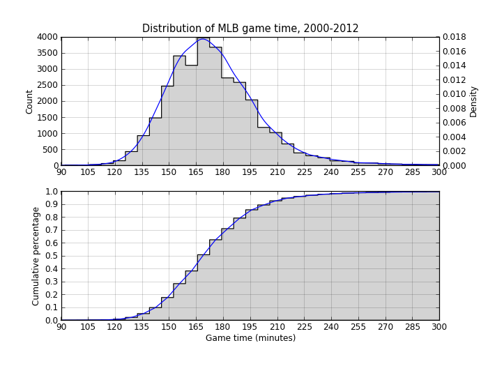
The two plots show what the descriptive statistics did: 70% of games are under three hours but it’s not uncommon for games to last three hours and fifteen minutes. Beyond that, it’s pretty uncommon.
Change in game times in the last 100 years
Now let’s look at how game times have changed over the years. First we eliminate all the games that weren’t complete in 51 or 54 innings to standardize the “game” were’re evaluating.
nine_innings = gamelog[gamelog.game_outs.isin([51, 54])]
nine_innings['year'] = nine_innings.apply(lambda x: x['dte'].year, axis=1)
nine_groupby_year = nine_innings.groupby('year')
mean_time_by_year = nine_groupby_year['game_time_min'].aggregate(np.mean)
fig = plt.figure()
p = mean_time_by_year.plot(figsize=(8, 4))
p.set_xlim(1915, 2015)
p.set_xlabel('Year')
p.set_ylabel('Game Time (minutes)')
p.set_title('Average MLB nine-inning game time since 1915')
p.set_xticks(range(1915, 2016, 10))
plt.savefig('game_time_by_year.png', dpi=87.5)
plt.savefig('game_time_by_year.svg')
plt.savefig('game_time_by_year.pdf')
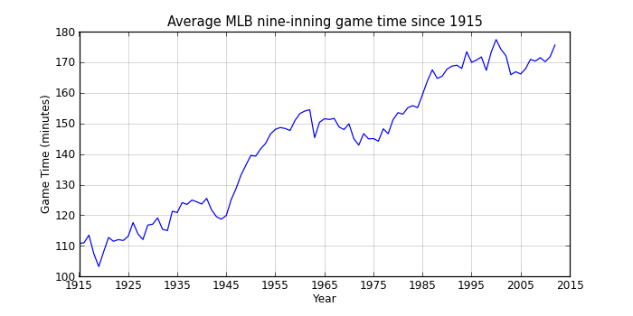
That shows a pretty clear upward trend interrupted by a slight decline between 1960 and 1975 (when offense was down across baseball). Since the mid-90s, game times have hovered around 2:50, so maybe MLB’s efforts at increasing the pace of the game have at least stopped what had been an almost continual rise in game times.
Attendance
I’ll be seeing a game at Wrigley Field, so let’s examine attendance at Wrigley.
Attendance is field 17, “Park ID” is field 16, but we can probably use Home team (field 6) = “CHN” for seasons after 1914 when it opened.
twenty_first[twenty_first['home_team'] == 'CHN']['attendance'].describe()
count     1053.000000
mean     37326.561254
std       5544.121773
min          0.000000
25%      36797.000000
50%      38938.000000
75%      40163.000000
max      55000.000000
We see the minimum is zero, which may indicate bad or missing data. Let’s look at all the games at Wrigley with less than 10,000 fans:
twenty_first[(twenty_first.home_team == 'CHN') &
             (twenty_first.attendance < 10000)][[
            'dte', 'visiting_team', 'home_team', 'visitor_score',
            'home_score', 'game_outs', 'day_night', 'attendance',
            'game_time_min']]
| dte | vis | hme | vis | hme | outs | day | att | game_time | |
|---|---|---|---|---|---|---|---|---|---|
| 172776 | 2000-06-01 | ATL | CHN | 3 | 5 | 51 | D | 5267 | 160 |
| 173897 | 2000-08-25 | LAN | CHN | 5 | 3 | 54 | D | 0 | 189 |
| 174645 | 2001-04-18 | PHI | CHN | 3 | 4 | 51 | D | 0 | 159 |
| 176290 | 2001-08-20 | MIL | CHN | 4 | 7 | 51 | D | 0 | 180 |
| 177218 | 2002-04-28 | LAN | CHN | 5 | 4 | 54 | D | 0 | 196 |
| 177521 | 2002-05-21 | PIT | CHN | 12 | 1 | 54 | N | 0 | 158 |
| 178910 | 2002-09-02 | MIL | CHN | 4 | 2 | 54 | D | 0 | 193 |
| 181695 | 2003-09-27 | PIT | CHN | 2 | 4 | 51 | D | 0 | 169 |
| 183806 | 2004-09-10 | FLO | CHN | 7 | 0 | 54 | D | 0 | 146 |
| 184265 | 2005-04-13 | SDN | CHN | 8 | 3 | 54 | D | 0 | 148 |
| 188186 | 2006-08-03 | ARI | CHN | 10 | 2 | 54 | D | 0 | 197 |
Looks like the zeros are just missing data because these games have relevant data for the other fields and it’s impossible to believe that not a single person was in the stands. We’ll get rid of them for the attendance analysis.
Now we’ll filter the games so we’re only looking at day games played at Wrigley where the attendance value is above zero, and group the data by day of the week.
groupby_dow = twenty_first[(twenty_first['home_team'] == 'CHN') &
           (twenty_first['day_night'] == 'D') &
           (twenty_first['attendance'] > 0)].groupby('day_of_week')
groupby_dow['attendance'].aggregate(np.mean).order()
day_of_week
Tue            34492.428571
Wed            35312.265957
Thu            35684.737864
Mon            37938.757576
Fri            38066.060976
Sun            38583.833333
Sat            39737.428571
Name: attendance
And plot it:
filtered = twenty_first[(twenty_first['home_team'] == 'CHN') &
                           (twenty_first['day_night'] == 'D') &
                           (twenty_first['attendance'] > 0)]
dows = {'Sun':0, 'Mon':1, 'Tue':2, 'Wed':3, 'Thu':4, 'Fri':5, 'Sat':6}
filtered['dow'] = filtered.apply(lambda x: dows[x['day_of_week']], axis=1)
filtered['attendance'] = filtered['attendance'] / 1000.0
fig = plt.figure()
d = filtered.boxplot(column='attendance', by='dow', figsize=(8, 4))
plt.suptitle('')
d.set_xlabel('Day of the week')
d.set_ylabel('Attendance (thousands)')
d.set_title('Wrigley Field attendance by day of the week, 2000-2012')
labels = ['Sun', 'Mon', 'Tue', 'Wed', 'Thu', 'Fri', 'Sat']
l = d.set_xticklabels(labels)
d.set_ylim(15, 45)
plt.savefig('attendance.png', dpi=87.5)
plt.savefig('attendance.svg') # lines don't show up?
plt.savefig('attendance.pdf')
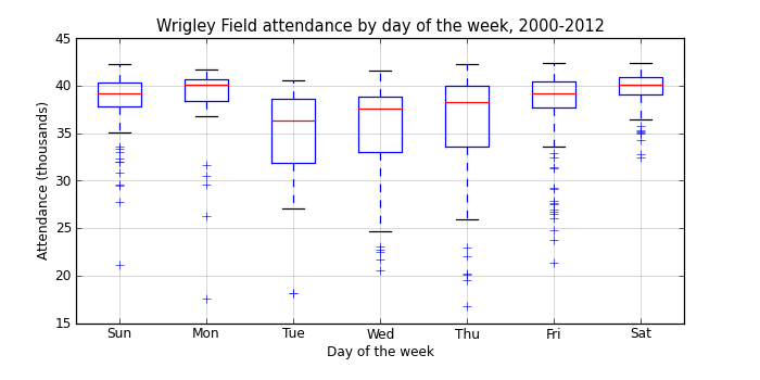
There’s a pretty clear pattern here, with increasing attendance from Tuesday through Monday, and larger variances in attendance during the week.
It’s a bit surprising that Monday games are as popular as Saturday games, especially since we’re only looking at day games. On any given Monday when the Cubs are at home, there’s a good chance that there will be fourty thousand people not showing up to work!