Introduction
I’ve been brewing beer since the early 90s, and since those days the number of hops available to homebrewers has gone from a handfull of varieties (Northern Brewer, Goldings, Fuggle, Willamette, Cluster) to well over a hundred. Whenever I go to my local brewing store I’m bewildered by the large variety of hops, most of which I’ve never heard of. I’m also not all that fond of super-citrusy hops like Cascade or it’s variants, so it is a challenge to find flavor and aroma hops that aren’t citrusy among the several dozen new varieties on display.
Most of the hops at the store are Yakima Chief – Hop Union branded, and they’ve got a great web site that lists all their varieties and has information about each hop. As convenient as a website can be, I’d rather have the data in a database where I can search and organize it myself. Since the data is all on the website, we can use a web scraping library to grab it and format it however we like.
One note: websites change all the time, so whenever the structure of a site changes, the code to grab the data will need to be updated. I originally wrote the code for this post a couple weeks ago, scraping data from the Hop Union web site. This morning, that site had been replaced with an entirely different Yakima Chief – Hop Union site and I had to completely rewrite the code.
rvest
I’m using the rvest package from Hadley Wickham and RStudio to do the work of pulling the data from each page. In the Python world, Beautiful Soup would be the library I’d use, but there’s a fair amount of data manipulation needed here and I felt like dplyr would be easier.
Process
First, load all the libraries we need.
library(rvest)       # scraping data from the web
library(dplyr)       # manipulation, filtering, grouping into tables
library(stringr)     # string functions
library(tidyr)       # creating columns from rows
library(RPostgreSQL) # dump final result to a PostgreSQL database
Next, we retrieve the data from the main page that has all the varieties listed on it, and extract the list of links to each hop. In the code below, we read the entire document into a variable, hop_varieties using the read_html function.
Once we’ve got the web page, we need to find the HTML nodes that contain links to the page for each individual hop. To do that, we use html_nodes(), passing a CSS selector to the function. In this case, we’re looking for a tags that have a class of card__name. I figured this out by looking at the raw source code from the page using my web browser’s inspection tools. If you right-click on what looks like a link on the page, one of the options in the pop-up menu is “inspect”, and when you choose that, it will show you the HTML for the element you clicked on. It can take a few tries to find the proper combination of tag, class, attribute or id to uniquely identify the things you want.
The YCH site is pretty well organized, so this isn’t too difficult. Once we’ve got the nodes, we extract the links by retrieving the href attribute from each one with html_attr().
hop_varieties <- read_html("http://ychhops.com/varieties")

hop_page_links <- hop_varieties %>%
    html_nodes("a.card__name") %>%
    html_attr("href")
Now we have a list of links to all the varieties on the page. It turns out that they made a mistake when they transitioned to the new site and the links all have the wrong host (ych.craft.dev). We can fix that by applying replacing the host in all the links.
fixed_links <- sapply(hop_page_links,
                     FUN=function(x) sub('ych.craft.dev',
                                         'ychhops.com', x)) %>%
    as.vector()
Each page will need to be loaded, the relevant information extracted, and the data formatted into a suitable data structure. I think a data frame is the best format for this, where each row in the data frame represents the data for a single hop and each column is a piece of information from the web page.
First we write a function the retrieves the data for a single hop and returns a one-row data frame with that data. Most of the data is pretty simple, with a single value for each hop. Name, description, type of hop, etc. Where it gets more complicated is the each hop can have more than one aroma category, and the statistics for each hop vary from one to the next. What we’ve done here is combine the aromas together into a single string, using the at symbol (@) to separate the parts. Since it’s unlikely that symbol will appear in the data, we can split it back apart later. We do the same thing for the other parameters, creating an @-delimited string for the items, and their values.
get_hop_stats <- function(p) {
    hop_page <- read_html(p)

    hop_name <- hop_page %>%
        html_nodes('h1[itemprop="name"]') %>%
        html_text()

    type <- hop_page %>%
        html_nodes('div.hop-profile__data div[itemprop="additionalProperty"]') %>%
        html_text()
    type <- (str_split(type, ' '))[[1]][2]

    region <- hop_page %>%
        html_nodes('div.hop-profile__data h5') %>%
        html_text()

    description <- hop_page %>%
        html_nodes('div.hop-profile__profile p[itemprop="description"]') %>%
        html_text()

    aroma_profiles <- hop_page %>%
        html_nodes('div.hop-profile__profile h3.headline a[itemprop="category"]') %>%
        html_text()

    aroma_profiles <- sapply(aroma_profiles,
                             FUN=function(x) sub(',$', '', x)) %>%
        as.vector() %>%
        paste(collapse="@")

    composition_keys <- hop_page %>%
        html_nodes('div.hop-composition__item') %>%
        html_text()

    composition_keys <- sapply(composition_keys,
                               FUN=function(x)
                                   tolower(gsub('[ -]', '_', x))) %>%
        as.vector() %>%
        paste(collapse="@")

    composition_values <- hop_page %>%
        html_nodes('div.hop-composition__value') %>%
        html_text() %>%
        paste(collapse="@")

    hop <- data.frame('hop'=hop_name, 'type'=type, 'region'=region,
                      'description'=description,
                      'aroma_profiles'=aroma_profiles,
                      'composition_keys'=composition_keys,
                      'composition_values'=composition_values)

}
With a function that takes a URL as input, and returns a single-row data frame, we use a common idiom in R to combine everything together. The inner-most lapply function will run the function on each of the fixed variety links, and each single-row data frame will then be combined together using rbind within do.call.
all_hops <- do.call(rbind,
                    lapply(fixed_links, get_hop_stats)) %>% tbl_df() %>%
    arrange(hop) %>%
    mutate(id=row_number())
At this stage we’ve retrieved all the data from the website, but some of it has been encoded in a less that useful format.
Data tidying
To tidy the data, we want to extract only a few of the item / value pairs of data from the data frame, alpha acid, beta acid, co-humulone and total oil. We also need to remove carriage returns from the description and remove the aroma column.
We split the keys and values back apart again using the @ symbol used earlier to combine them, then use unnest to create duplicate columns with each of the key / value pairs in them. spread pivots these up into columns such that the end result has one row per hop with the relevant composition values as columns in the tidy data set.
hops <- all_hops %>%
    arrange(hop) %>%
    mutate(description=gsub('\\r', '', description),
           keys=str_split(composition_keys, "@"),
           values=str_split(composition_values, "@")) %>%
    unnest(keys, values) %>%
    spread(keys, values) %>%
    select(id, hop, type, region, alpha_acid, beta_acid, co_humulone, total_oil, description)

kable(hops %>% select(id, hop, type, region, alpha_acid) %>% head())
| id | hop | type | region | alpha_acid |
|---|---|---|---|---|
| 1 | Admiral | Bittering | United Kingdom | 13 - 16% |
| 2 | Ahtanum™ | Aroma | Pacific Northwest | 3.5 - 6.5% |
| 3 | Amarillo® | Aroma | Pacific Northwest | 7 - 11% |
| 4 | Aramis | Aroma | France | 7.9 - 8.3% |
| 5 | Aurora | Dual | Slovenia | 7 - 9.5% |
| 6 | Bitter Gold | Dual | Pacific Northwest | 12 - 14.5% |
For the aromas we have a one to many relationship where each hop has one or more aroma categories associated. We could fully normalize this by created an aroma table and a join table that connects hop and aroma, but this data is simple enough that I just created the join table itself. We’re using the same str_split / unnest method we used before, except that in this case we don't want to turn those into columns, we want a separate row for each hop × aroma combination.
hops_aromas <- all_hops %>%
    select(id, hop, aroma_profiles) %>%
    mutate(aroma=str_split(aroma_profiles, "@")) %>%
    unnest(aroma) %>%
    select(id, hop, aroma)
Saving and exporting
Finally, we save the data and export it into a PostgreSQL database.
save(list=c("hops", "hops_aromas"),
     file="ych_hops.rdata")

beer <- src_postgres(host="dryas.swingleydev.com", dbname="beer",
                     port=5434, user="cswingle")

dbWriteTable(beer$con, "ych_hops", hops %>% data.frame(), row.names=FALSE)
dbWriteTable(beer$con, "ych_hops_aromas", hops_aromas %>% data.frame(), row.names=FALSE)
Usage
I created a view in the database that combines all the aroma categories into a Postgres array type using this query. I also use a pair of regular expressions to convert the alpha acid string into a Postgres numrange.
CREATE VIEW ych_basic_hop_data AS
SELECT ych_hops.id, ych_hops.hop, array_agg(aroma) AS aromas, type,
    numrange(
        regexp_replace(alpha_acid, '([0-9.]+).*', E'\\1')::numeric,
        regexp_replace(alpha_acid, '.*- ([0-9.]+)%', E'\\1')::numeric,
        '[]') AS alpha_acid_percent, description
FROM ych_hops
    INNER JOIN ych_hops_aromas USING(id)
GROUP BY ych_hops.id, ych_hops.hop, type, alpha_acid, description
ORDER BY hop;
With this, we can, for example, find US aroma hops that are spicy, but without citrus using the ANY() and ALL() array functions.
SELECT hop, region, type, aromas, alpha_acid_percent
FROM ych_basic_hop_data
WHERE type = 'Aroma' AND region = 'Pacific Northwest' AND 'Spicy' = ANY(aromas)
AND 'Citrus' != ALL(aromas) ORDER BY alpha_acid_percent;

     hop    |      region       | type  |            aromas            | alpha_acid_percent
 -----------+-------------------+-------+------------------------------+--------------------
  Crystal   | Pacific Northwest | Aroma | {Floral,Spicy}               | [3,6]
  Hallertau | Pacific Northwest | Aroma | {Floral,Spicy,Herbal}        | [3.5,6.5]
  Tettnang  | Pacific Northwest | Aroma | {Earthy,Floral,Spicy,Herbal} | [4,6]
  Mt. Hood  | Pacific Northwest | Aroma | {Spicy,Herbal}               | [4,6.5]
  Santiam   | Pacific Northwest | Aroma | {Floral,Spicy,Herbal}        | [6,8.5]
  Ultra     | Pacific Northwest | Aroma | {Floral,Spicy}               | [9.2,9.7]
Code
The RMarkdown version of this post, including the code can be downloaded from GitHub:
Boil
Over the past month and a half I’ve brewed four beers, starting with Piper’s Irish-American Ale , and culminating with Mr. Silly IPA which is in the middle of the mash right now. We’re less than a week from when we normally get the first snowfall that lasts until spring, so this will likely be the end of my 2012 brewing effort.
My normal process is to make a yeast starter from a Wyeast smack-pack or White Labs tube, pitch that into the first batch, and a week later siphon the chilled wort of the second batch onto the yeast cake from the first.
I didn’t have time to make a starter for Piper’s, so I just smacked the pack (Wyeast 1084, Irish Ale) on brew day and assumed there’d be enough healthy yeast to make quick work of the 1.049 wort. After two days of no visible activity, I began to worry that the yeast in the pack had been killed at some point before I bought it. Finally on day three, something finally started to happen and the beer has since fermented successfully.
The second batch was a 1.077 old ale I poured into my Old Alexi solera ale keg (recipe is here). It kicked off almost immediately and was probably 90% fermented within 24 hours due to the thick, healthy yeast from fermenting Piper’s.
During both fermentations I kept track of the temperatures in the fermentation chamber (a fridge with heater on a temperature controller) and in the wort using my Arduino data logger. A graph of the two fermentations is below:
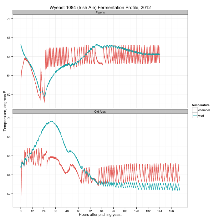
You can see the activity of the temperature controller on the temperature in the chamber (the orange line), clicking the heater on and off within 4 degrees of the set temperature. For Piper’s (the top plot) I started with the chamber at 64°F, but almost immediately bumped it up to 66°F when the wort temperature crashed. After 24 hours, something finally started happening in the wort, with a peak temperature (and fermentation) on day three. When I transferred the wort from primary to secondary on day seven, there was still active fermentation.
Compare this with the second beer. The wort started at 65°F, and immediately took off, peaking a little over 24 hours later. By day three, fermentation was over. I dropped the fermentation chamber temperature from 66°F to 64°F after the first day.
What did I learn? First: always make a yeast starter. It’s no fun waiting several days for fermentation to finally take off, and during that lull the wort is vulnerable to other infections that could damage the flavor. Second: don’t panic, especially with a yeast that has a reputation of starting slowly like Wyeast 1084. It usually works out in the end. More often than not, the Papazian “relax, enjoy a homebrew” mantra really is the way to approach brewing.
I used a starter for last week’s batch (Taiga Dog AK Mild, White Labs WLP007, Dry English Ale) and it was visibly fermenting within a day and a half. Mr. Silly will undoubtedly have a similar fermentation temperature curve like Old Alexi above after I transfer the wort onto the Taiga Dog yeast cake.

Tallys, Caslon, and Jenson
I took Friday off from work and brewed my first batch of beer in quite a long time. It’s a brown porter named Crazy Kittens Porter. As should be obvious, it’s named after our three crazy kittens Caslon, Tallys and Jenson, pictured on the right. This time around I developed the recipe using the BrewPal iPhone app, trusting all the measurements and temperatures to the app. We’ll see how well it does. My favorite part of the app is the “style” tab, which shows you what styles your recipe conforms to and to what degree.
Normally I do everything out in the red cabin, but I had the wood stove cranking so I heated the strike and spare water on the wood stove and drained the mash in the kitchen (shown below). It was nice to be able to do that stuff in the house and to avoid burning fossil fuels for the wort production. As usual, I boiled and chilled the wort outside and set the fermenter in the old fridge out in the red cabin. It’s bubbling away now.
I plan to brew another batch of Devil Dog on top of the yeast cake from this batch. This is an excellent way to save some money on yeast, and the second batch normally gets a very explosive start from the massive population of healthy yeast.

Sparging with kittens

Protein after the boil
Spent some of yesterday brewing a batch of Bavarian hefeweizen. It’s a light, easy drinking summer beer that preserves the unique flavors of the Bavarian wheat beer yeasts. Most American varieties of hefeweizen use a cleaner, less flavorful American yeast. My original version of this beer was named after the shed I build to house our water tank in the old house. Now that we’ve moved and have a new shed, the beer has been re-christened “New Shed Hefeweizen.”
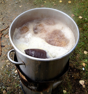
The beer has six pounds of base malt—two pounds of 6-row and four pounds of 2-row organic pale malt in this case—and six pounds of malted wheat. Wheat malt contains a lot of protein, as does the 6-row malt. As I mentioned in my post about Piper’s Red Ale, protein causes haze in the final beer and can affect it’s long-term stability. In the case of a hefeweizen, the haze is a feature of the style, and because it’s a summer “session-style” beer, it’ll get consumed more quickly than a typical ale. So all the protein shouldn’t be a problem and will contribute to a nice thick head on the finished beer. You can see all the protein floating around in the wort (it’s the white stuff in the photo that looks like the eggs in egg-drop soup). Most of the big chunks get filtered out in the pot as the wort is chilled, but even with the gross removal, there’s still a lot left over in the fermenter.
My last batch of beer, Devil Dog turned into a comedy of errors. The mash and boil went perfectly, but when chilling I accidentally left the stopcock on my fermenting bucket open. Lost a couple gallons of wort into the snow. After fermentation was finished and it was in the keg, one of my new serving lines had a loose bolt on the keg connector. Not only did this cause all the remaining beer to leak out inside my kegerator (three gallons of it), but I completely drained my CO2 tank. So this time around, I paid very careful attention to everything I was doing.

Chilling the wort
The mash, boil, and chilling went well. Mashing a grain bill that’s 50% wheat is always a little nerve-wracking because wheat has no husks to help in filtration, and as anyone who had made bread by hand knows, wheat plus water equals a very sticky substance. My mill does a good job of preserving the barley husks, and I didn’t have any extraction issues when sparging. I wound up with an excess of wort, however, so I had to boil it quite a bit longer to get down to five gallons. The final beer might be a bit maltier as a result, because of the additional carmalization of the sugars in the pot. I bumped up the hops slightly in an attempt to offset this.
Chilling was a bit of an experiment. I pulled thirty gallons of water from Goldstream Creek and used that in a closed loop through my plate chiller to chill the wort. It’s in the blue barrel on the right side of the image. The temperature at the start was around 50°F, and that wasn’t quite cool enough to drain the kettle with the valve all the way open. But I got it down to a pitching temperature of 70°F, which is about right for a hefeweizen.
A true hefeweizen yeast is an interesting strain because you can control the flavors from the yeast by changing the fermentation temperature. Like Belgian beers, a Bavarian hefeweizen comes with lots of flavors that would be considered serious defects in a British (or worse, American) ale. At cooler temperatures (cooler than 65°F), you’ll get more banana flavors, and warmer fermentation encourages clove tones. I tend to prefer the banana flavor, but at lower temperatures you’re always risking a sluggish or incomplete fermentation. This time around, I’m hoping to keep fermentation closer to 68°F, which should yield a nice dry beer with a good balance of banana and clove flavors.
Assuming I don’t pump all the beer into my kegerator again, I should know how it turned out in four to six weeks.

Fermentation, day one
Yesterday I brewed my ninth batch of Piper’s Irish-American Red Ale, based on a recipe from Jeff Renner posted in the Homebrew Digest. It’s an easy drinking, low alcohol (4.0—4.7%) red ale. My version isn’t a traditional Irish Red Ale because it’s got six-row malt and corn in it, but this is likely to have been the combination of grains used by early Irish immigrants to the United States. When the English first colonized North America, two-row barley for brewing was imported from Britain. Six-row barley grew much better in our climate, but it is higher in protein than two-row barley, which results in a cloudy beer, and one which spoils more readily (especially without refrigeration). The solution to this problem is to replace some of the six-row barley starches with other types of starch like corn. The high-protein barley will readily convert the starches in the corn to the simple sugars that yeast can consume, and the total amount of protein in the final product will be reduced. It was a great adaptation to the native strain of barley grown in early America.
We don’t have to worry about that now, of course, but I enjoy renewing some older brewing traditions. This batch is a little over 40% British two-row pale malt, 30% American six-row malted barley, and 20% flaked maize. There’s some flaked barley for head retention, and crystal 60 and chocolate malt to produce the malt flavor and color of a red ale.

Andrea’s photo of Piper, The Toothbrush Dog
I was trying out a new transfer pump on this batch, as my previous one was damaged by ice the last time I brewed. I’d left my water supply barrel outside overnight and when the very cold water hit the pump, it froze. The other issue with the old pump was that it would shut down when the outlet flow was constricted too much, a problem during chilling because I use a ball valve to limit the flow of cold water into the plate chiller. The new pump screamed right through the constricted flow and I got the wort from boiling to 64°F without any problems this time. I would have preferred a pitching temperature closer to 68°F, but I’d made a yeast starter, and the low wort temperature didn’t seem to slow it down at all. This morning there was a thick head of yeasty foam on the surface (as you can see in the photo).
While I was brewing, Andrea took some of the dogs to Mush for Kids where Piper was the Toothbrush Dog. She walked around with a backpack filled with toothbrushes for the kids who went to the event. Check out Andrea’s blog for more details and photos.