
Koidern
Yesterday we lost Koidern to complications from laryngeal paralysis. Koidern came to us in 2006 from Andrea’s mushing partner who thought she was too “ornery.” It is true that she wouldn’t hesitate to growl at a dog or cat who got too close to her food bowl, and she was protective of her favorite bed, but in every other way she was a very sweet dog. When she was younger she loved to give hugs, jumping up on her hind legs and wrapping her front legs around your waist. She was part Saluki, which made her very distinctive in Andrea’s dog teams and she never lost her beautiful brown coat, perky ears, and curled tail. I will miss her continual energy in the dog yard racing around after the other dogs, how she’d pounce on dog bones and toss them around, “smash” the cats, and the way she’d bark right before coming into the house as if to announce her entrance.
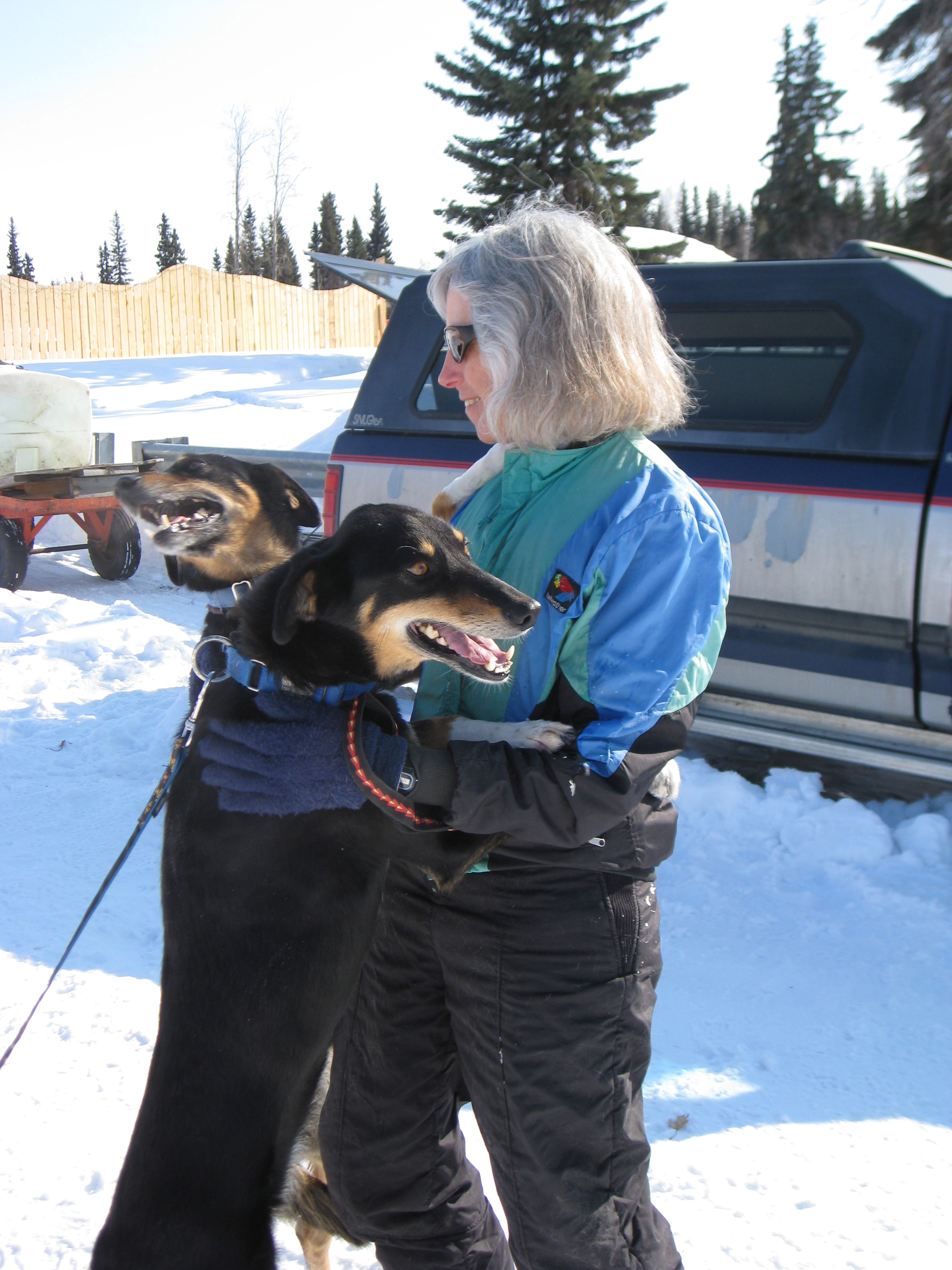
Koidern hug (with her sister Kluane and Carol Kaynor)
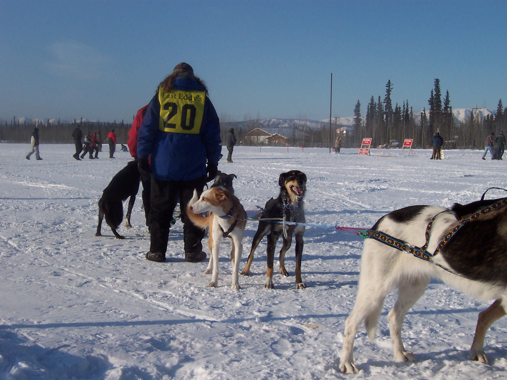
Koidern in Tok, with Piper and Buddy
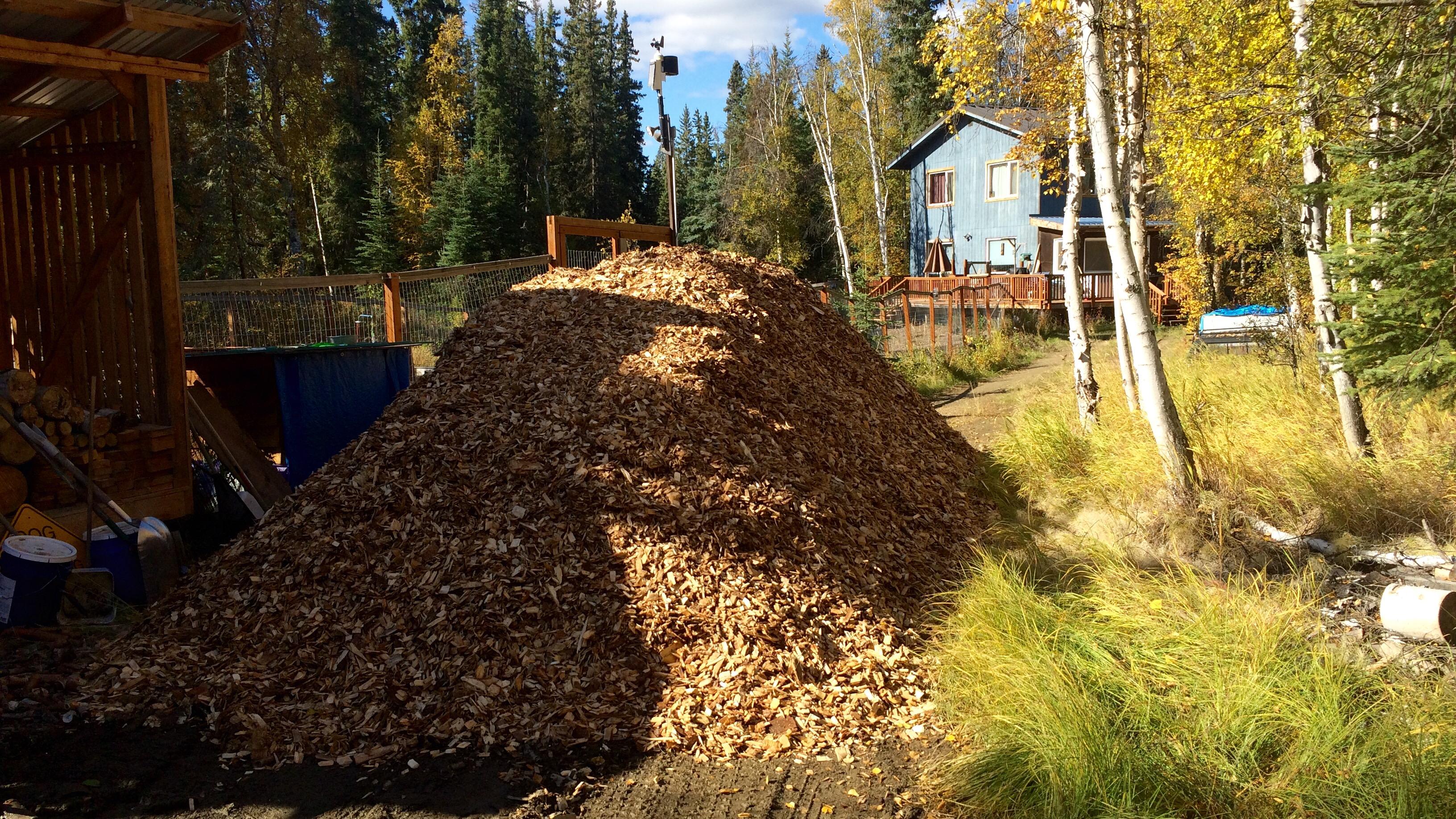
Thirty yards of wood chips
Every couple years we cover our dog yard with a fresh layer of wood chips from the local sawmill, Northland Wood. This year I decided to keep closer track of how much effort it takes to move all 30 yards of wood chips by counting each wheelbarrow load, recording how much time I spent, and by using a heart rate monitor to keep track of effort.
The image below show the tally board. Tick marks indicate wheelbarrow-loads, the numbers under each set of five were the number of minutes since the start of each bout of work, and the numbers on the right are total loads and total minutes. I didn’t keep track of time, or heart rate, for the first set of 36 loads.

It’s not on the chalkboard, but my heart rate averaged 96 beats per minute for the first effort on Saturday morning, and 104, 96, 103, and 103 bpm for the rest. That averages out to 100.9 beats per minute.
For the loads where I was keeping track of time, I averaged 3 minutes and 12 seconds per load. Using that average for the 36 loads on Friday afternoon, that means I spent around 795 minutes, or 13 hours and 15 minutes moving and spreading 248 wheelbarrow-loads of chips.
Using a formula found in [Keytel LR, et al. 2005. Prediction of energy expenditure from heart rate monitoring during submaximal exercise. J Sports Sci. 23(3):289-97], I calculate that I burned 4,903 calories above the amount I would have if I’d been sitting around all weekend. To put that in perspective, I burned 3,935 calories running the Equinox Marathon in September, 2013.
As I was loading the wheelbarrow, I was mentally keeping track of how many pitchfork-loads it took to fill the wheelbarrow, and the number hovered right around 17. That means there are about 4,216 pitchfork loads in 30 yards of wood chips.
To summarize: 30 yards of wood chips is equivalent to 248 wheelbarrow loads. Each wheelbarrow-load is 0.1209 yards, or 3.26 cubic feet. Thirty yards of wood chips is also equivalent to 4,216 pitchfork loads, each of which is 0.19 cubic feet. It took me 13.25 hours to move and spread it all, or 3.2 minutes per wheelbarrow-load, or 11 seconds per pitchfork-load.
One final note: this amount completely covered all but a few square feet of the dog yard. In some places the chips were at least six inches deep, and in others there’s just a light covering of new over old. I don’t have a good measure of the yard, but if I did, I’d be able to calculate the average depth of the chips. My guess is that it is around 2,500 square feet, which is what 30 yards would cover to an average depth of 4 inches.
I spent some time this weekend playing with a couple interesting new R packages that should help with some of the difficulty manipulating data with the base packages. Getting data into a format appropriate for plotting or running statistical models often seems to take more time than anything else, and the process can be very frustrating because of seemingly non-sensical error messages from R.
R guru Hadley Wickham has written some of the best packages for data manipulation (reshape2, plyr) and plotting (ggplot2). He’s got a new pair of packages (tidyr and dplyr) and a theory of getting data into the proper format (http://vita.had.co.nz/papers/tidy-data.pdf) that look very promising.
A couple other tools I wanted to look at include a new way of piping data from one operation to another (magrittr), which is a basic part of the Unix philosophy of having many tools that do one thing well and stringing them together to do neat things, and an interactive graphic package, ggvis, that should be really good for data investigation.
For this investigation, I’m looking at the names of our dogs, past and present, and how popular they are as people names in the United States. This data comes from the Social Security Administration and is available in the R package babynames.
install.packages("babynames")
library(babynames)
head(babynames)
Source: local data frame [6 x 5]

year sex      name    n       prop
1 1880   F      Mary 7065 0.07238359
2 1880   F      Anna 2604 0.02667896
3 1880   F      Emma 2003 0.02052149
4 1880   F Elizabeth 1939 0.01986579
5 1880   F    Minnie 1746 0.01788843
6 1880   F  Margaret 1578 0.01616720
The data has the number of registrations (n) and proportion of total registrations (prop) for each year from 1880 through 2013 for all name and sex combinations.
What I want to see is how popular out dog names are. All of our dogs have been adopted, but some we chose names for them (Nika, Piper, Kiva), and the rest came with names we didn’t change (Deuce, Buddy, Koidern, Lennier, Martin, Monte and the second Piper). Dog mushers often choose a theme for a litter of puppies, which accounts for some of the unusual names (Deuce came from a litter of classic cars, Lennier came from a litter of Babylon 5 character names, Koidern from a litter of Yukon River tributary names).
So what I want to do is subset the babynames database to just the names of our dogs, combine male and female names together, and plot the popularity of these names over time.
Here’s how that’s done using the magrittr pipe operator (%>%):
library(dplyr)
library(magrittr)

dog_names <- babynames %>%
   filter(name %in% c("Nika", "Piper", "Buddy", "Koidern", "Deuce",
                     "Kiva", "Lennier", "Martin", "Monte")) %>%
   group_by(year, name) %>%
   summarise(prop=sum(prop)) %>%
   transform(name=factor(name)) %>%
   ungroup() %>%
   arrange(name, year)
We are assigning the result of all the pipes to dog_names. In order, we take the babynames data set and filter it by our dog’s names. Then we group by year and name, and summarize the proportion values by sum. At this point we have data with just our dog’s names, with the proportions of both male and female baby names combined. Next, we convert the name variable to a factor, remove the grouping, and sort by name and year.
Here’s what it looks like now:
> head(dog_names)
year  name         prop
1 1893 Buddy 4.130866e-05
2 1894 Buddy 5.604573e-05
3 1896 Buddy 8.522045e-05
4 1898 Buddy 3.784782e-05
5 1899 Buddy 4.340353e-05
6 1900 Buddy 6.167015e-05
Now we’ve got tidy filtered and sorted data, so let’s plot it. I’ve been using ggplot2 for many years, and I think it’s the best way to produce publication quality figures. But usually you want to do some investigation of the data before doing that, and doing this in ggplot2 involves many cycles of code manipulation, plotting, viewing in order to see what you’ve got and how you want the final version to look.
ggvis is a new package that displays data interactively in a web browser. It also supports the pipe operator, so you can pipe the data directly into the plotting routine. It’s somewhat similar to ggplot2, but has some new conventions that are required in order to handle interactivity. Here’s a plot of my dog names data. The first part is the same as before, but I’m piping the result directly into ggivs.
library(ggvis)
babynames %>%
   filter(name %in% c("Nika", "Piper", "Buddy", "Koidern", "Deuce",
                     "Kiva", "Lennier", "Martin", "Monte")) %>%
   group_by(year, name) %>%
   summarise(prop=sum(prop)) %>%
   transform(name=factor(name)) %>%
   ungroup() %>%
   arrange(name, year) %>%
   ggvis(~year, ~prop, stroke=~name, fill=~name) %>%
   # layer_lines(strokeWidth:=2) %>%
   layer_points(size:=15) %>%
   add_axis("x", title="Year", format="####") %>%
   add_axis("y", title="Proportion of total names", title_offset=50) %>%
   add_legend(c("stroke", "fill"), title="Name")
Popularity of our dog names, ggvis version
Typically, I prefer to include lines and points in a timeseries plot like this, but I couldn't get ggvis to color the lines and the points without some very strange fill artifacts.
Here’s what I’d consider to be a high quality version of this, generated with ggplot:
library(ggplot2)
library(scales)

q <- ggplot(data=dog_names, aes(x=year, y=prop, colour=name)) +
         geom_point(size=1.75) +
         geom_line() +
         theme_bw() +
         scale_colour_brewer(palette="Set1") +
         scale_x_continuous(name="Year", breaks=pretty_breaks(n=10)) +
         scale_y_continuous(name="Proportion of total names", breaks=pretty_breaks(n=10))
rescale <- 0.50
svg("dog_names_ggplot2.svg", height=9*rescale, width=16*rescale)
print(q)
dev.off()
Popularity of our dog names, ggplot2 version
I think the two plots are pretty similar, and I’m impressed with how good the ggvis plot looks and how similar the language is to ggplot2. And I really like the pipe operator compared with a long list of individual statements or the way you add things together with ggplot2.
Both plots suffer from having too many groups (seven), which means it becomes difficult to interpret the colors on the plot. Choosing a good palette is key to this, and is one of those parts of figure production that can really take a long time. I don’t think my choices in the ggplot2 version is optimal, but I got tired of looking. The other problem is the collection of dog names with very low proportions among human babies. Because they’re all overlapping near the axis, this data is obscured. Both problems could be solved by stacking two plots on top of each other, one with the more popular names (Martin, Piper, Buddy and Monte) and one with the less popular ones (Deuce, Kiva, Nika) using different scales for the proportion axis.
What does the plot show? Among our dog’s names, Martin was the most popular, but it’s popularity has been declining since the 60s, and the name Piper has been increasing since 2000. Both Monte and Buddy were popular in the past, but have declined to low levels recently.
For reference, here are the number of babies in 2013 that were given names matching those of our dogs:
babynames %>%
   filter(name %in% c("Nika", "Piper", "Buddy", "Koidern", "Deuce",
                     "Kiva", "Lennier", "Martin", "Monte")
         & year==2013) %>%
   group_by(year, name) %>%
   summarise(n=sum(n)) %>%
   transform(name=factor(name)) %>%
   ungroup() %>%
   arrange(desc(n))

year   name    n
1 2013  Piper 3166
2 2013 Martin 1330
3 2013  Monte   81
4 2013   Nika   67
5 2013  Buddy   21
6 2013   Kiva   18
7 2013  Deuce    5
I spent most of October and November building a dog barn for the dogs. Our two newest dogs (Lennier and Monte) don’t have sufficient winter coats to be outside when it’s colder than ‒15°F. A dog barn is a heated space with large, comfortable, locking dog boxes inside. The dogs sleep inside at night and are pretty much in the house with us when we’re home, but when we’re at work or out in town, the dogs can go into the barn to stay warm on cold days.
You can view the photos of the construction on my photolog
Along with the dog boxes we’ve got a monitoring and control system in the barn:
- An Arduino board that monitors the temperature (DS18B20 sensor) and humidity (SHT15) in the barn and controls an electric heater through a Power Tail II.
- A BeagleBone Black board running Linux which reads the data from the Arduino board and inserts it into a database, and can change the set temperature that the Arduino uses to turn the heater on and off (typically we leave this set at 30°F, which means the heater comes on at 28 and goes off at 32°F).
- An old Linksys WRT-54G router (running DD-WRT) which connect to the wireless network in the house and connects to BeagleBone setup via Ethernet.
The system allows us to monitor the conditions inside the barn in real-time, and to change the temperature. It is a little less robust than the bi-metallic thermostat we were using initially, but as long as the Arduino has power, it is able to control the heat even if the BeagleBone or wireless router were to fail, and is far more accurate. It’s also a lot easier to keep track of how long the heater is on if we’re turning it on and off with our monitoring system.
Thursday we got an opportunity to see what happens when all the dogs are in there at ‒15°F. They were put into their boxes around 10 AM, and went outside at 3:30 PM. The windows were closed.
Here’s a series of plots showing what happened (PDF version)
The top plot shows the temperature in the barn. As expected, the temperature varies from 28°F, when the heater comes on, to a bit above 32°F when the heater goes off. There are obvious spikes in the plot when the heater comes on and rapidly warms the building. Interestingly, once the dogs were settled into the barn, the heater didn’t come on because the dogs were keeping the barn warm themselves. The temperature gradually rose while they were in there.
The next plot is the relative humidity. In addition to heating the barn, the dogs were filling it with moisture. It’s clear that we will need to deal with all that moisture in the future. We plan on experimenting with a home-built heat recovery ventilator (HRV) that is based on alternating sheets of Coroplast plastic. The idea is that warm air from inside travels through one set of layers to the outside, cold air from outside passes through the other set of layers and is heated on it’s way in by the exiting warm air. Until that’s done, our options are to leave the two windows cracked to allow the moisture to escape (with some of the warm air, of course) or to use a dehumidifier.
The bar chart shows the number of minutes the power was on for the interval shown. Before the dogs went into the barn the heater was coming on for about 15 minutes, then was off for 60 minutes before coming back on again. As the temperature cools outside, the interval when the heater is off decreases. Again, this plot shows the heater stopped coming on once the dogs were in the barn.
The bottom plot is the outside temperature.
So far the barn is a great addition to the property, and the dogs really seem to like it, charging into the barn and into their boxes when it’s cold outside. I’m looking forward to experimenting with the HRV and seeing what happens under similar conditions but with the windows slighly open, or when the outside temperatures are much colder.
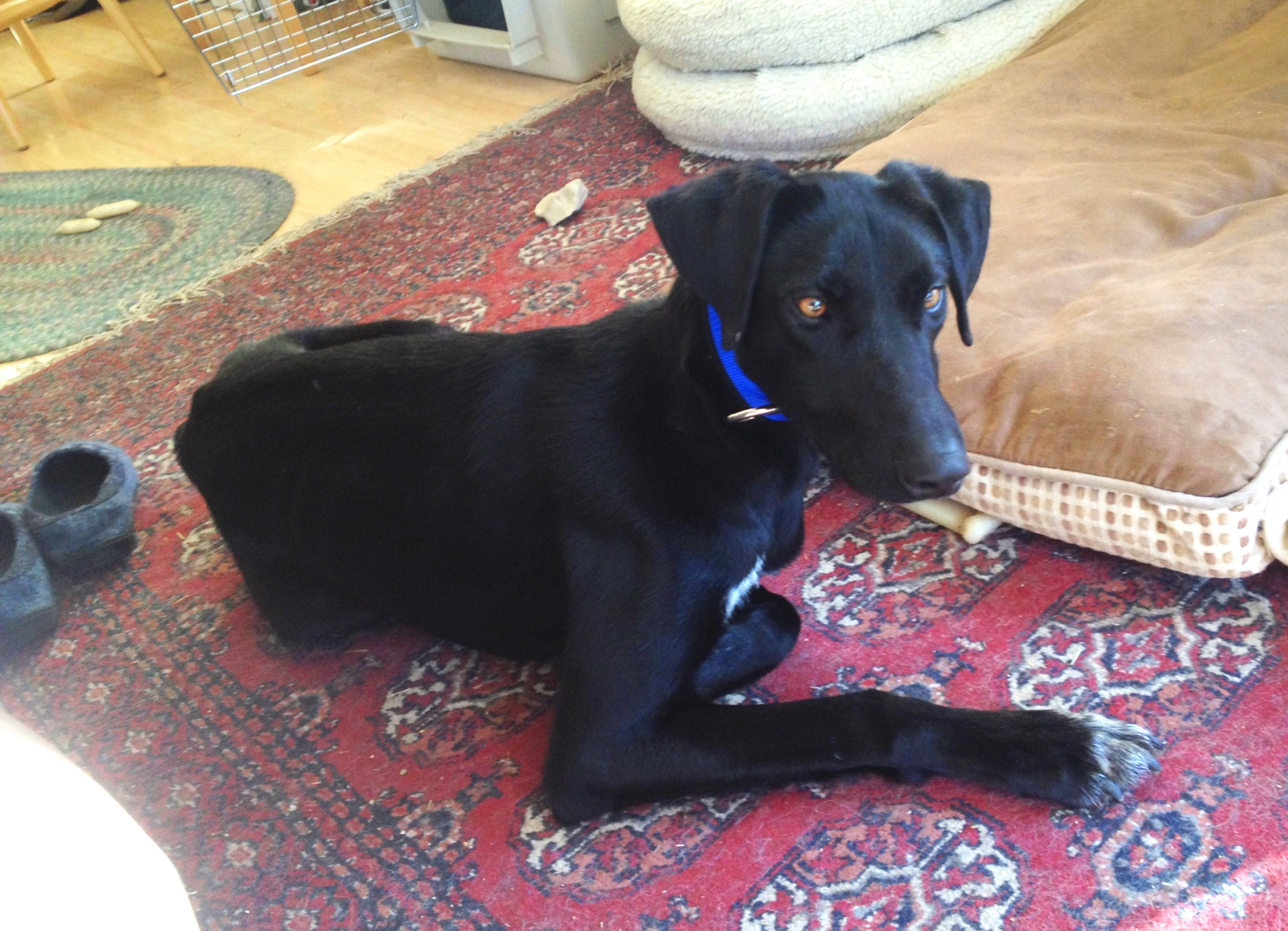
Lennier
Long before Nika and Piper died, we had planned on taking one of the dogs that Andrea’s mushing parter didn’t want, a large hound mix named Lennier (the litter was named after characters in the Babylon 5 television series). Even though we are still mourning our loss, we didn’t feel like it was a reason not to give another dog a chance in our home. He’s a yearling dog, and is a big boy, a couple inches taller than Buddy, and quite a bit longer. At the moment he is all legs, but he may still grow into his body.
Last night was a pretty taxing affair, with him too curious and excited to relax for even a minute, and a trio of cats very scared of the new resident. He has been better today, and is even sleeping on the floor at my feet right now. He appears to be mostly curious about the cats, but unfortunately, his only real experience with them so far is when they’re running away at warp speed, tails puffed.
In time, I’m sure he’ll get used to his new life, and will become part of the family. Welcome, Lennier!