Introduction
The Alaska Department of Transportation is working on updating their bicycling and pedestrian master plan for the state and their web site mentions Alaska as having high percentages of bicycle and pedestrian commuters relative to the rest of the country. I’m interested because I commute to work by bicycle (and occasionally ski or run) every day, either on the trails in the winter, or the roads in the summer. The company I work for (ABR) pays it’s employees $3.50 per day for using non-motorized means of transportation to get to work. I earned more than $700 last year as part of this program and ABR has paid it’s employees almost $40K since 2009 not to drive to work.
The Census Bureau keeps track of how people get to work in the American Community Survey, easily accessible from their web site. We’ll use this data to see if Alaska really does have higher than average rates of non-motorized commuters.
Data
The data comes from FactFinder. I chose ‘American Community Survey’ from the list of data sources near the bottom, searched for ‘bicycle’, chose ‘Commuting characteristics by sex’ (Table S0801), and added the ‘All States within United States and Puerto Rico’ as the Geography of interest. The site generates a zip file containing the data as a CSV file along with several other informational files. The code for extracting the data appears at the bottom of this post.
The data are percentages of workers 16 years and over and their means of transportation to work. Here’s a table showing the top 10 states ordered by the combination of bicycling and walking percentage.
| state | total | motorized | carpool | public_trans | walk | bicycle | |
|---|---|---|---|---|---|---|---|
| 1 | District of Columbia | 358,150 | 38.8 | 5.2 | 35.8 | 14.0 | 4.1 |
| 2 | Alaska | 363,075 | 80.5 | 12.6 | 1.5 | 7.9 | 1.1 |
| 3 | Montana | 484,043 | 84.9 | 10.4 | 0.8 | 5.6 | 1.6 |
| 4 | New York | 9,276,438 | 59.3 | 6.6 | 28.6 | 6.3 | 0.7 |
| 5 | Vermont | 320,350 | 85.1 | 8.2 | 1.3 | 5.8 | 0.8 |
| 6 | Oregon | 1,839,706 | 81.4 | 10.2 | 4.8 | 3.8 | 2.5 |
| 7 | Massachusetts | 3,450,540 | 77.6 | 7.4 | 10.6 | 5.0 | 0.8 |
| 8 | Wyoming | 289,163 | 87.3 | 10.0 | 2.2 | 4.6 | 0.6 |
| 9 | Hawaii | 704,914 | 80.9 | 13.5 | 7.0 | 4.1 | 0.9 |
| 10 | Washington | 3,370,945 | 82.2 | 9.8 | 6.2 | 3.7 | 1.0 |
Alaska has the second highest rates of walking and biking to work behind the District of Columbia. The table is an interesting combination of states with large urban centers (DC, New York, Oregon, Massachusetts) and those that are more rural (Alaska, Montana, Vermont, Wyoming).
Another way to rank the data is by combining all forms of transportation besides single-vehicle motorized transport (car pooling, public transportation, walking and bicycling).
| state | total | motorized | carpool | public_trans | walk | bicycle | |
|---|---|---|---|---|---|---|---|
| 1 | District of Columbia | 358,150 | 38.8 | 5.2 | 35.8 | 14.0 | 4.1 |
| 2 | New York | 9,276,438 | 59.3 | 6.6 | 28.6 | 6.3 | 0.7 |
| 3 | Massachusetts | 3,450,540 | 77.6 | 7.4 | 10.6 | 5.0 | 0.8 |
| 4 | New Jersey | 4,285,182 | 79.3 | 7.5 | 11.6 | 3.3 | 0.3 |
| 5 | Alaska | 363,075 | 80.5 | 12.6 | 1.5 | 7.9 | 1.1 |
| 6 | Hawaii | 704,914 | 80.9 | 13.5 | 7.0 | 4.1 | 0.9 |
| 7 | Oregon | 1,839,706 | 81.4 | 10.2 | 4.8 | 3.8 | 2.5 |
| 8 | Illinois | 6,094,828 | 81.5 | 7.9 | 9.3 | 3.0 | 0.7 |
| 9 | Washington | 3,370,945 | 82.2 | 9.8 | 6.2 | 3.7 | 1.0 |
| 10 | Maryland | 3,001,281 | 82.6 | 8.9 | 9.0 | 2.6 | 0.3 |
Here, the states with large urban centers come out higher because of the number of commuters using public transportation. Despite very low availability of public transportation, Alaska still winds up 5th on this list because of high rates of car pooling, in addition to walking and bicycling.
Map data
To look at regional patterns, we can make a map of the United States colored by non-motorized transportation percentage. This can be a little challenging because Alaska and Hawaii are so far from the rest of the country. What I’m doing here is loading the state data, transforming the data to a projection that’s appropriate for Alaska, and moving Alaska and Hawaii closer to the lower-48 for display. Again, the code appears at the bottom.
You can see that non-motorized transportation is very low throughout the deep south, and tends to be higher in the western half of the country, but the really high rates of bicycling and walking to work are isolated. High Vermont next to low New Hampshire, or Oregon and Montana split by Idaho.
Urban and rural, median age of the population
What explains the high rates of non-motorized commuting in Alaska and the other states at the top of the list? Urbanization is certainly one important factor explaining why the District of Columbia and states like New York, Oregon and Massachusetts have high rates of walking and bicycling. But what about Montana, Vermont, and Wyoming?
Age of the population might have an effect as well, as younger people are more likely to walk and bike to work than older people. Alaska has the second youngest population (33.3 years) in the U.S. and DC is third (33.8), but the other states in the top five (Utah, Texas, North Dakota) don’t have high non-motorized transportation.
So it’s more complicated that just these factors. California is a good example, with a combination of high urbanization (second, 95.0% urban), low median age (eighth, 36.2) and great weather year round, but is 19th for non-motorized commuting. Who walks in California, after all?
Conclusion
I hope DOT comes up with a progressive plan for improving opportunities for pedestrian and bicycle transportation in Alaska They’ve made some progress here in Fairbanks; building new paths for non-motorized traffic; but they also seem blind to the realities of actually using the roads and paths on a bicycle. The “bike path” near my house abruptly turns from asphalt to gravel a third of the way down Miller Hill, and the shoulders of the roads I commute on are filled with deep snow in winter, gravel in spring, and all manner of detritus year round. Many roads don’t have a useable shoulder at all.
Code
library(tidyverse)  # data import, manipulation
library(knitr)      # pretty tables
library(rpostgis)   # PostGIS support
library(rgdal)      # geographic transformation
library(maptools)   # geographic transformation
library(viridis)    # color blind color palette

# Read the heading
heading <- read_csv('ACS_15_1YR_S0801.csv', n_max = 1) %>% names()

# Read the data
s0801 <- read_csv('ACS_15_1YR_S0801.csv', col_names = FALSE, skip = 2)

names(s0801) <- heading

# Extract only the columns we need, add state postal codes
commute <- s0801 %>%
    transmute(state = `GEO.display-label`,
              total = HC01_EST_VC01,
              motorized = HC01_EST_VC03,
              carpool = HC01_EST_VC05,
              public_trans = HC01_EST_VC10,
              walk = HC01_EST_VC11,
              bicycle = HC01_EST_VC12) %>%
    filter(state != 'Puerto Rico') %>%
    mutate(state_postal = c('AL', 'AK', 'AZ', 'AR', 'CA', 'CO', 'CT',
                            'DE', 'DC', 'FL', 'GA', 'HI', 'ID', 'IL',
                            'IN', 'IA', 'KS', 'KY', 'LA', 'ME', 'MD',
                            'MA', 'MI', 'MN', 'MS', 'MO', 'MT', 'NE',
                            'NV', 'NH', 'NJ', 'NM', 'NY', 'NC', 'ND',
                            'OH', 'OK', 'OR', 'PA', 'RI', 'SC', 'SD',
                            'TN', 'TX', 'UT', 'VT', 'VA', 'WA', 'WV',
                            'WI', 'WY'))

# Print top ten tables
kable(commute %>% select(-state_postal) %>%
      arrange(desc(walk + bicycle)) %>% head(n = 10),
  format.args = list(big.mark = ","),
  row.names = TRUE)

kable(commute %>% select(-state_postal) %>%
      arrange(motorized) %>% head(n = 10),
  format.args = list(big.mark = ","),
  row.names = TRUE)

# Connect to the database with the state layer
layers <- src_postgres(host = "localhost",
                             dbname = "layers")

states <- pgGetGeom(layers$con, c("public", "states"),
                    geom = "wkb_geometry", gid = "ogc_fid")

# Transform to srid 3338 (Alaska Albers)
states_3338 <- spTransform(states, CRS("+proj=aea +lat_1=55 +lat_2=65 +lat_0=50
                                       +lon_0=-154 +x_0=0 +y_ 0=0 +ellps=GRS80
                                       +towgs84=0,0,0,0,0,0,0 +units=m
                                       +no_defs"))

# Convert to a data frame suitable for ggplot, move AK and HI
ggstates <- fortify(states_3338, region = "state") %>%
    filter(id != 'PR') %>%
    inner_join(commute, by = (c("id" = "state_postal"))) %>%
    mutate(lat = ifelse(state == 'Hawaii', lat + 2300000, lat),
           long = ifelse(state == 'Hawaii', long + 2000000, long),
           lat = ifelse(state == 'Alaska', lat + 1000000, lat),
           long = ifelse(state == 'Alaska', long + 2000000, long))

# Plot it
p <- ggplot() + geom_polygon(data = ggstates, colour = "black",
                        aes(x = long, y = lat, group = group,
                            fill = bicycle + walk)) +
    coord_fixed(ratio = 1) +
    scale_fill_viridis(name = "Non-motorized\n commuters (%)",
                       option = "plasma",
                       limits = c(0, 9), breaks = seq(0, 9, 3)) +
    theme_void() +
    theme(legend.position = c(0.9, 0.2))

width <- 16
height <- 9
resize <- 0.75

svg("non_motorized_commute_map.svg", width = width*resize, height = height*resize)
print(p)
dev.off()
pdf("non_motorized_commute_map.pdf", width = width*resize, height = height*resize)
print(p)
dev.off()

# Urban and rural percentages by state
heading <- read_csv('../urban_rural/DEC_10_SF1_P2.csv', n_max = 1) %>% names()

dec10 <- read_csv('../urban_rural/DEC_10_SF1_P2.csv', col_names = FALSE, skip = 2)

names(dec10) <- heading

urban_rural <- dec10 %>%
    transmute(state = `GEO.display-label`,
              total = D001,
              urban = D002,
              rural = D005) %>%
    filter(state != 'Puerto Rico') %>%
    mutate(urban_percentage = urban / total * 100)

# Median age by state
heading <- read_csv('../age_sex/ACS_15_1YR_S0101.csv', n_max = 1) %>% names()

s0101 <- read_csv('../age_sex/ACS_15_1YR_S0101.csv', col_names = FALSE, skip = 2)

names(s0101) <- heading

age <- s0101 %>%
    transmute(state = `GEO.display-label`,
              median_age = HC01_EST_VC35) %>%
    filter(state != 'Puerto Rico')

# Do urban percentage and median age explain anything about
# non-motorized transit?
census_data <- commute %>%
    inner_join(urban_rural, by = "state") %>%
    inner_join(age, by = "state") %>%
    select(state, state_postal, walk, bicycle, urban_percentage, median_age) %>%
    mutate(non_motorized = walk + bicycle)

u <- ggplot(data = census_data,
       aes(x = urban_percentage, y = non_motorized)) +
    geom_text(aes(label = state_postal))

svg("urban.svg", width = width*resize, height = height*resize)
print(u)
dev.off()

a <- ggplot(data = census_data,
       aes(x = median_age, y = non_motorized)) +
    geom_text(aes(label = state_postal))

svg("age.svg", width = width*resize, height = height*resize)
print(a)
dev.off()

# Not significant:
model = lm(data = census_data,
           non_motorized ~ urban_percentage + median_age)

# Only significant because of DC (a clear outlier)
model = lm(data = census_data,
           non_motorized ~ urban_percentage * median_age)

1991 contacts
Yesterday I was going through my journal books from the early 90s to see if I could get a sense of how much bicycling I did when I lived in Davis California. I came across the list of my network contacts from January 1991 shown in the photo. I had an email, bitnet and uucp address on the UC Davis computer system. I don’t have any record of actually using these, but I do remember the old email clients that required lines be less than 80 characters, but which were unable to edit lines already entered.
I found the statistics for 109 of my bike rides between April 1991 and June 1992, and I think that probably represents most of them from that period. I moved to Davis in the fall of 1990 and left in August 1993, however, and am a little surprised I didn’t find any rides from those first six months or my last year in California.
I rode 2,671 miles in those fifteen months, topping out at 418 miles in June 1991. There were long gaps in the record where I didn’t ride at all, but when I rode, my average weekly mileage was 58 miles and maxed out at 186 miles.
To put that in perspective, in the last seven years of commuting to work and riding recreationally, my highest monthly mileage was 268 miles (last month!), my average weekly mileage was 38 miles, and the farthest I’ve gone in a week was 81 miles.
The road biking season is getting near to the end here in Fairbanks as the chances of significant snowfall on the roads rises dramatically, but I hope that next season I can push my legs (and hip) harder and approach some of the mileage totals I reached more than twenty years ago.

Skiing home
This year I’ve made a serious effort to improve my physical fitness. I started lifting weights in August, and worked hard to commute to work as much as I could by bicycle (6.7 miles each way) or ski (4.1 miles). I commuted on 102 days this year, which is 40% of the possible work days in the year. I also spent a lot of time out on the trails with our now 15-year old dog, Nika. In May, I set up a standing desk at work, and as I’ll demonstrate below, this is a significant improvement over spending all those hours sitting, at least for energy consumption. As a result of all this, I feel like I am in the best shape of my life, and that makes me feel good as I enter middle age.
Here’s the summary of what I did this year (details on the calculations appear below):
| Activity | Miles | Hours | Speed | Energy |
|---|---|---|---|---|
| Treadmill | 8.98 | 1.58 | 5.62 | 925 |
| Skiing | 268.35 | 54.25 | 4.98 | 27,685 |
| Bicycling | 960.22 | 69.67 | 13.86 | 38,606 |
| Hiking | 201.06 | 81.56 | 2.53 | 28,750 |
| Skating | 3.49 | 0.75 | 4.65 | 236 |
| Lifting | 56.10 | 19,775 | ||
| TOTAL | 1,442 | 263.91 | 115,976 |
The other thing I did was start standing up at my desk at work. I spent 1,258 hours at my desk after I started standing. According to the Compendium of Physical Activities, standing at work consumes 2.3 metabolic equivalent units (MET). This is the ratio of work metabolic rate over resting metabolic rate, which would be 1.0 MET. Thus, standing uses an additional 1.3 MET over resting. Sitting at a desk is 1.5 MET, which means standing adds 0.8 MET.
To use these numbers, you need an estimate of your resting metabolic rate. Using the Mifflin et al. equation on this page I get 1,691 Kcal/day, or 70.5 Kcal per hour for my height, weight, and age. For those 1,258 hours standing at work I burned an additional 71 thousand calories: 1,258 • 0.8 • 70.5 = 70,951 Kcal (the “calories” reported on food labels are technically kilocalories (Kcal) in energy units). That’s a lot of energy, just by standing instead of sitting.
The energy values in the table above were also calculated using the same methods. I fiddled with the tabular values from the compendium and got the following approximations:
- Running MET = 1.653 • speed (mph)
- Skiing = ((speed - 2.5) / 2) + 7
- Bicycling = speed - 5
- Hiking = 6
- Skating = 5.5
- Lifting = 6
Despite the amount of energy consumed by standing instead of sitting at work, I think there is a real benefit to the more intense exercises listed in the table. These strengthen and build skeletal and cardiovascular muscle in ways that simply standing all day don’t.
When all the numbers are totaled, I burned an extra 512 calories (318 exercising, 194 standing) each day in 2011. That’s certainly worth a beer or two, and I look and feel better for it even drinking them!
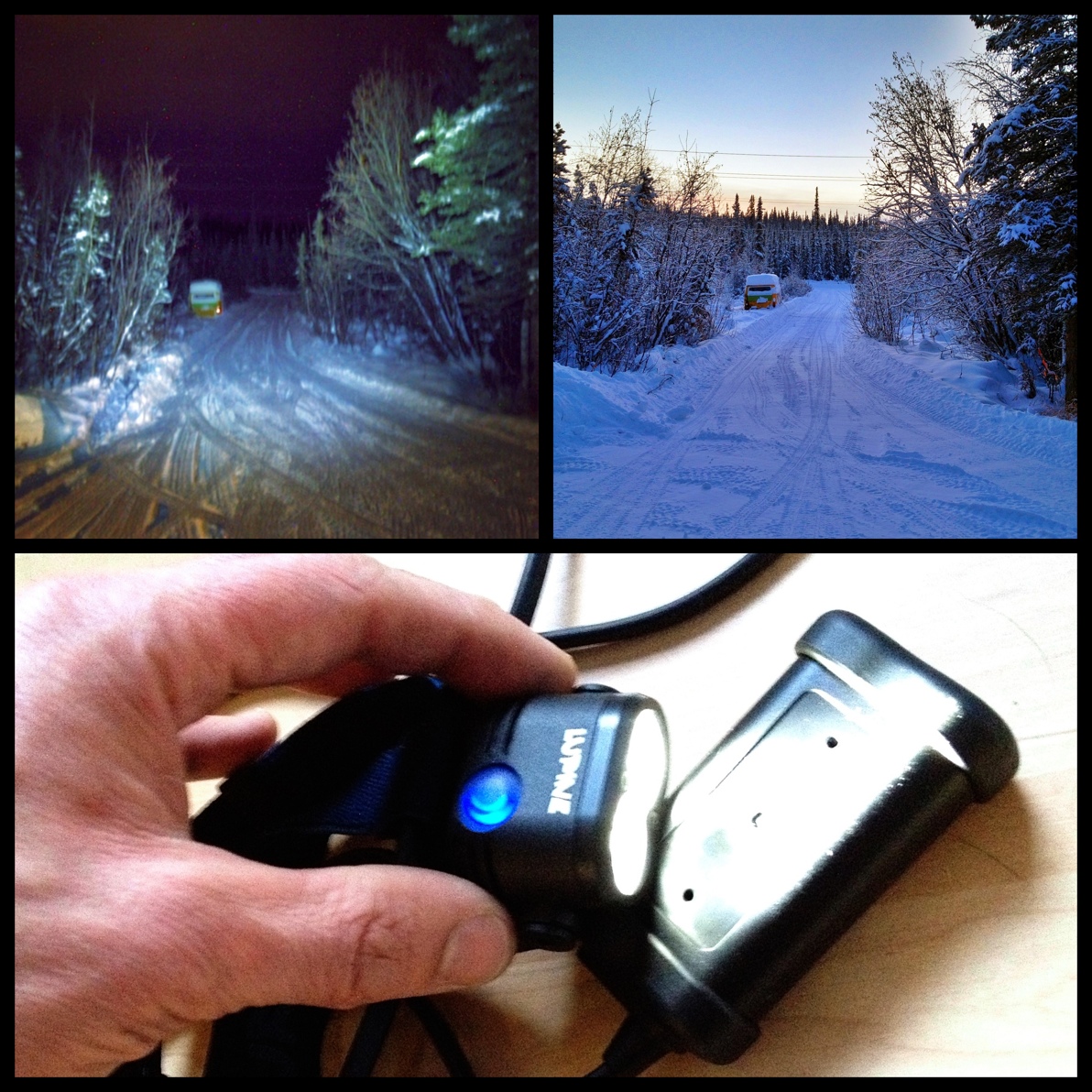
Lupine Pico X
This year I've made a real effort to commute to work on my bicycle or skis as much as I can. It's a 6.7 mile bicycle ride and 4.1 miles on the ski trails. A lot of this commuting is done in the dark, and until last week I'd been using a Petzl headlamp with an incandescent bulb, powered by four C-cell batteries. It's adequate when the batteries are fresh, and there aren't any cars around or moose on the trail. Unfortunately, when I really need to see where a moose has gone, or when a car is blasting its headlights in my face, I might as well not even have the light. Car headlights are so much brighter than the headlamp that the road literally disappears for as long as a minute after they've passed while my eyes readjust.
Not anymore. Last weekend I bought a 750 lumen, rechargeable LED headlamp made by Lupine. It's the Pico X model, and comes with a charger, headlamp strap, and a extension cord for the battery. As you can see in the bottom photo above, the battery pack is quite small, as is the lamp itself.
The upper photos attempt to demonstrate how much light it puts out (left side is at night with the headlamp, right side is a daytime photo). It's about 250 feet from where I'm standing to the line of trees across the street from our driveway, and they are clearly illuminated by the headlamp (although it's hard to see in the photo). Basically, everything I can see during the daylight photo is visible with the headlamp at its brightest.
The spotlight is easily bright enough to compete with a car headlight, even with its high-beams on, and according to the documentation, the battery will power the headlamp at this brightness for two hours before needing a recharge. The lamp also has two lower brightness modes, with longer battery life.
The whole package is expensive—$360—but it really makes a huge difference in how much you can see around you. The company I work for (ABR) pays us to use alternative forms of transportation to get to work, and my efforts this year will just about pay for the headlamp. A perfect way to spend my benefit and improve my future non-motorized travels.
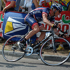
Lance Armstrong. photo by eugene
I was disappointed to hear that the government (and 60 Minutes) is now going after bicycling legend Lance Armstrong. Just like with Barry Bonds, confidential grand jury testimony is somehow available to the media, and our tax dollars are being wasted pursing former top athletes instead of actually trying to solve the problems facing our society.
Like cancer. Lance Armstrong is a cancer survivor, and through his LiveStrong foundation he’s raised over $400 million dollars for medical research to fight the disease. What’s the gain in taking him down now?
When asked how his belief in God helped him beat cancer, he replied:
Everyone should believe in something, and I believe in surgery, chemotherapy, and my doctors.
Yep. Science. Among other things, we use it to improve vision, repair broken bones, cure diseases, manufacture high tech bicycles, rebuild arms and legs, and, yes, improve our body’s ability to perform. I suppose the line between allowed (alcohol, caffeine, tobacco, Lasix eye surgery, artificial nutritional supplements, Tommy John surgery) and forbidden (marijuana, amphetamines, steroids, artificial limbs, blood doping) has to be drawn somewhere, but it all feels pretty arbitrary. And rarely does it seem like bringing down our heros (McGwire, Bonds, Sosa, Pettitte, Clemens, and now Armstrong) is doing any of us any good for all the expense it costs us.
Note: Andy Pettitte was never one of my heroes, but he was the winningest pitcher of the 2000s, and, apparently, a steroid user.