Introduction
I’ve been brewing beer since the early 90s, and since those days the number of hops available to homebrewers has gone from a handfull of varieties (Northern Brewer, Goldings, Fuggle, Willamette, Cluster) to well over a hundred. Whenever I go to my local brewing store I’m bewildered by the large variety of hops, most of which I’ve never heard of. I’m also not all that fond of super-citrusy hops like Cascade or it’s variants, so it is a challenge to find flavor and aroma hops that aren’t citrusy among the several dozen new varieties on display.
Most of the hops at the store are Yakima Chief – Hop Union branded, and they’ve got a great web site that lists all their varieties and has information about each hop. As convenient as a website can be, I’d rather have the data in a database where I can search and organize it myself. Since the data is all on the website, we can use a web scraping library to grab it and format it however we like.
One note: websites change all the time, so whenever the structure of a site changes, the code to grab the data will need to be updated. I originally wrote the code for this post a couple weeks ago, scraping data from the Hop Union web site. This morning, that site had been replaced with an entirely different Yakima Chief – Hop Union site and I had to completely rewrite the code.
rvest
I’m using the rvest package from Hadley Wickham and RStudio to do the work of pulling the data from each page. In the Python world, Beautiful Soup would be the library I’d use, but there’s a fair amount of data manipulation needed here and I felt like dplyr would be easier.
Process
First, load all the libraries we need.
library(rvest)       # scraping data from the web
library(dplyr)       # manipulation, filtering, grouping into tables
library(stringr)     # string functions
library(tidyr)       # creating columns from rows
library(RPostgreSQL) # dump final result to a PostgreSQL database
Next, we retrieve the data from the main page that has all the varieties listed on it, and extract the list of links to each hop. In the code below, we read the entire document into a variable, hop_varieties using the read_html function.
Once we’ve got the web page, we need to find the HTML nodes that contain links to the page for each individual hop. To do that, we use html_nodes(), passing a CSS selector to the function. In this case, we’re looking for a tags that have a class of card__name. I figured this out by looking at the raw source code from the page using my web browser’s inspection tools. If you right-click on what looks like a link on the page, one of the options in the pop-up menu is “inspect”, and when you choose that, it will show you the HTML for the element you clicked on. It can take a few tries to find the proper combination of tag, class, attribute or id to uniquely identify the things you want.
The YCH site is pretty well organized, so this isn’t too difficult. Once we’ve got the nodes, we extract the links by retrieving the href attribute from each one with html_attr().
hop_varieties <- read_html("http://ychhops.com/varieties")

hop_page_links <- hop_varieties %>%
    html_nodes("a.card__name") %>%
    html_attr("href")
Now we have a list of links to all the varieties on the page. It turns out that they made a mistake when they transitioned to the new site and the links all have the wrong host (ych.craft.dev). We can fix that by applying replacing the host in all the links.
fixed_links <- sapply(hop_page_links,
                     FUN=function(x) sub('ych.craft.dev',
                                         'ychhops.com', x)) %>%
    as.vector()
Each page will need to be loaded, the relevant information extracted, and the data formatted into a suitable data structure. I think a data frame is the best format for this, where each row in the data frame represents the data for a single hop and each column is a piece of information from the web page.
First we write a function the retrieves the data for a single hop and returns a one-row data frame with that data. Most of the data is pretty simple, with a single value for each hop. Name, description, type of hop, etc. Where it gets more complicated is the each hop can have more than one aroma category, and the statistics for each hop vary from one to the next. What we’ve done here is combine the aromas together into a single string, using the at symbol (@) to separate the parts. Since it’s unlikely that symbol will appear in the data, we can split it back apart later. We do the same thing for the other parameters, creating an @-delimited string for the items, and their values.
get_hop_stats <- function(p) {
    hop_page <- read_html(p)

    hop_name <- hop_page %>%
        html_nodes('h1[itemprop="name"]') %>%
        html_text()

    type <- hop_page %>%
        html_nodes('div.hop-profile__data div[itemprop="additionalProperty"]') %>%
        html_text()
    type <- (str_split(type, ' '))[[1]][2]

    region <- hop_page %>%
        html_nodes('div.hop-profile__data h5') %>%
        html_text()

    description <- hop_page %>%
        html_nodes('div.hop-profile__profile p[itemprop="description"]') %>%
        html_text()

    aroma_profiles <- hop_page %>%
        html_nodes('div.hop-profile__profile h3.headline a[itemprop="category"]') %>%
        html_text()

    aroma_profiles <- sapply(aroma_profiles,
                             FUN=function(x) sub(',$', '', x)) %>%
        as.vector() %>%
        paste(collapse="@")

    composition_keys <- hop_page %>%
        html_nodes('div.hop-composition__item') %>%
        html_text()

    composition_keys <- sapply(composition_keys,
                               FUN=function(x)
                                   tolower(gsub('[ -]', '_', x))) %>%
        as.vector() %>%
        paste(collapse="@")

    composition_values <- hop_page %>%
        html_nodes('div.hop-composition__value') %>%
        html_text() %>%
        paste(collapse="@")

    hop <- data.frame('hop'=hop_name, 'type'=type, 'region'=region,
                      'description'=description,
                      'aroma_profiles'=aroma_profiles,
                      'composition_keys'=composition_keys,
                      'composition_values'=composition_values)

}
With a function that takes a URL as input, and returns a single-row data frame, we use a common idiom in R to combine everything together. The inner-most lapply function will run the function on each of the fixed variety links, and each single-row data frame will then be combined together using rbind within do.call.
all_hops <- do.call(rbind,
                    lapply(fixed_links, get_hop_stats)) %>% tbl_df() %>%
    arrange(hop) %>%
    mutate(id=row_number())
At this stage we’ve retrieved all the data from the website, but some of it has been encoded in a less that useful format.
Data tidying
To tidy the data, we want to extract only a few of the item / value pairs of data from the data frame, alpha acid, beta acid, co-humulone and total oil. We also need to remove carriage returns from the description and remove the aroma column.
We split the keys and values back apart again using the @ symbol used earlier to combine them, then use unnest to create duplicate columns with each of the key / value pairs in them. spread pivots these up into columns such that the end result has one row per hop with the relevant composition values as columns in the tidy data set.
hops <- all_hops %>%
    arrange(hop) %>%
    mutate(description=gsub('\\r', '', description),
           keys=str_split(composition_keys, "@"),
           values=str_split(composition_values, "@")) %>%
    unnest(keys, values) %>%
    spread(keys, values) %>%
    select(id, hop, type, region, alpha_acid, beta_acid, co_humulone, total_oil, description)

kable(hops %>% select(id, hop, type, region, alpha_acid) %>% head())
| id | hop | type | region | alpha_acid |
|---|---|---|---|---|
| 1 | Admiral | Bittering | United Kingdom | 13 - 16% |
| 2 | Ahtanum™ | Aroma | Pacific Northwest | 3.5 - 6.5% |
| 3 | Amarillo® | Aroma | Pacific Northwest | 7 - 11% |
| 4 | Aramis | Aroma | France | 7.9 - 8.3% |
| 5 | Aurora | Dual | Slovenia | 7 - 9.5% |
| 6 | Bitter Gold | Dual | Pacific Northwest | 12 - 14.5% |
For the aromas we have a one to many relationship where each hop has one or more aroma categories associated. We could fully normalize this by created an aroma table and a join table that connects hop and aroma, but this data is simple enough that I just created the join table itself. We’re using the same str_split / unnest method we used before, except that in this case we don't want to turn those into columns, we want a separate row for each hop × aroma combination.
hops_aromas <- all_hops %>%
    select(id, hop, aroma_profiles) %>%
    mutate(aroma=str_split(aroma_profiles, "@")) %>%
    unnest(aroma) %>%
    select(id, hop, aroma)
Saving and exporting
Finally, we save the data and export it into a PostgreSQL database.
save(list=c("hops", "hops_aromas"),
     file="ych_hops.rdata")

beer <- src_postgres(host="dryas.swingleydev.com", dbname="beer",
                     port=5434, user="cswingle")

dbWriteTable(beer$con, "ych_hops", hops %>% data.frame(), row.names=FALSE)
dbWriteTable(beer$con, "ych_hops_aromas", hops_aromas %>% data.frame(), row.names=FALSE)
Usage
I created a view in the database that combines all the aroma categories into a Postgres array type using this query. I also use a pair of regular expressions to convert the alpha acid string into a Postgres numrange.
CREATE VIEW ych_basic_hop_data AS
SELECT ych_hops.id, ych_hops.hop, array_agg(aroma) AS aromas, type,
    numrange(
        regexp_replace(alpha_acid, '([0-9.]+).*', E'\\1')::numeric,
        regexp_replace(alpha_acid, '.*- ([0-9.]+)%', E'\\1')::numeric,
        '[]') AS alpha_acid_percent, description
FROM ych_hops
    INNER JOIN ych_hops_aromas USING(id)
GROUP BY ych_hops.id, ych_hops.hop, type, alpha_acid, description
ORDER BY hop;
With this, we can, for example, find US aroma hops that are spicy, but without citrus using the ANY() and ALL() array functions.
SELECT hop, region, type, aromas, alpha_acid_percent
FROM ych_basic_hop_data
WHERE type = 'Aroma' AND region = 'Pacific Northwest' AND 'Spicy' = ANY(aromas)
AND 'Citrus' != ALL(aromas) ORDER BY alpha_acid_percent;

     hop    |      region       | type  |            aromas            | alpha_acid_percent
 -----------+-------------------+-------+------------------------------+--------------------
  Crystal   | Pacific Northwest | Aroma | {Floral,Spicy}               | [3,6]
  Hallertau | Pacific Northwest | Aroma | {Floral,Spicy,Herbal}        | [3.5,6.5]
  Tettnang  | Pacific Northwest | Aroma | {Earthy,Floral,Spicy,Herbal} | [4,6]
  Mt. Hood  | Pacific Northwest | Aroma | {Spicy,Herbal}               | [4,6.5]
  Santiam   | Pacific Northwest | Aroma | {Floral,Spicy,Herbal}        | [6,8.5]
  Ultra     | Pacific Northwest | Aroma | {Floral,Spicy}               | [9.2,9.7]
Code
The RMarkdown version of this post, including the code can be downloaded from GitHub:
Since the middle of 2010 we’ve been monitoring the level of Goldstream Creek for the National Weather Service by measuring the distance from the top of our bridge to the surface of the water or ice. In 2012 the Creek flooded and washed the bridge downstream. We eventually raised the bridge logs back up onto the banks and resumed our measurements.
This winter the Creek had been relatively quiet, with the level hovering around eight feet below the bridge. But last Friday, we awoke to more than four feet of water over the ice, and since then it's continued to rise. This morning’s reading had the ice only 3.17 feet below the surface of the bridge.
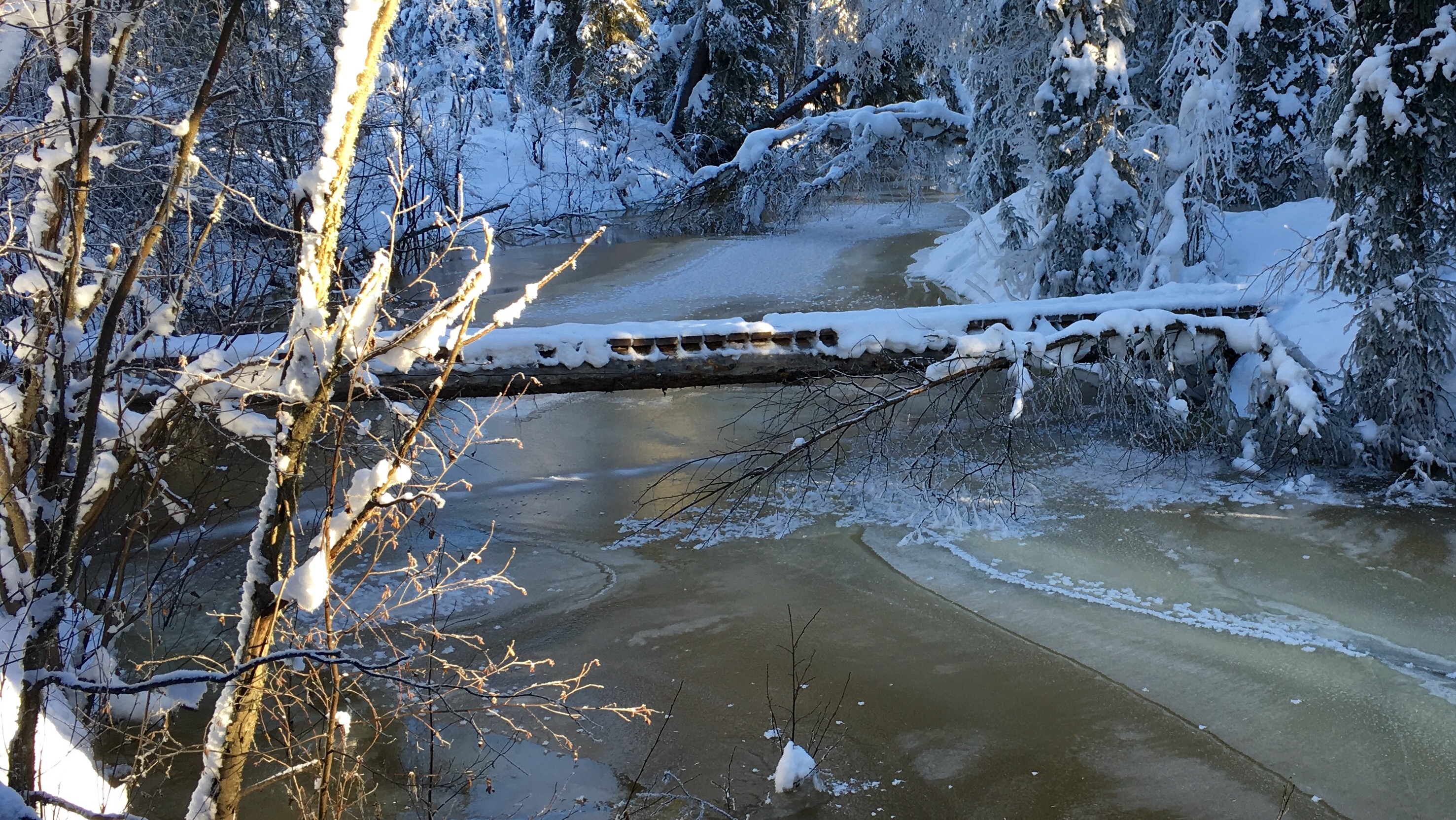
Overflow within a few feet of the bridge
Water also entered the far side of the slough, and is making it’s way around the loop, melting the snow covering the old surface. Even as the main channel stops rising and freezes, water moves closer to the dog yard from the slough.
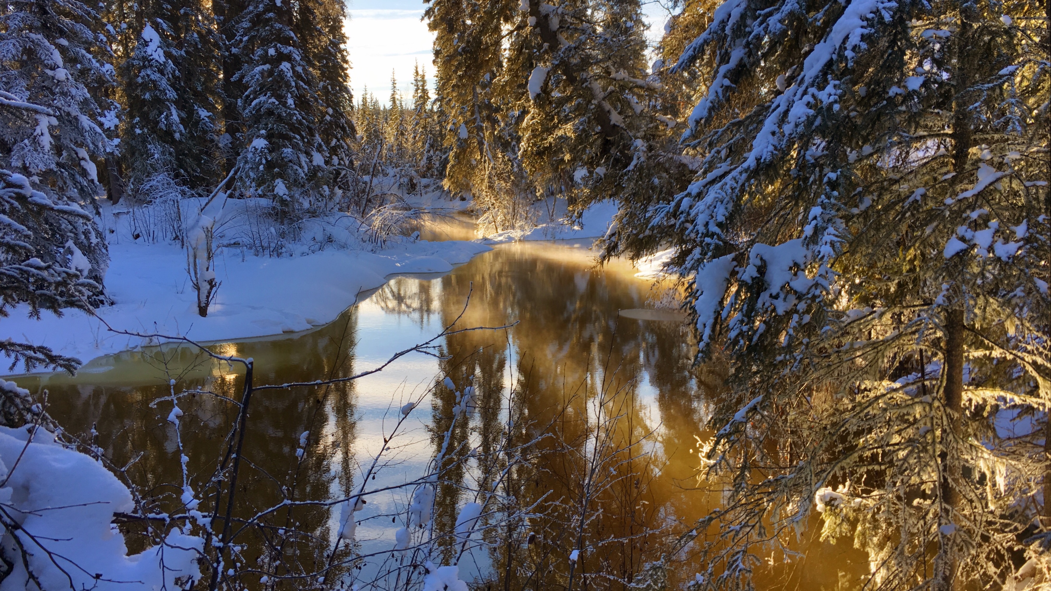
Water entering the slough
One of my longer commutes to work involves riding east on the Goldstream Valley trails, crossing the Creek by Ballaine Road, then riding back toward the house on the north side of the Creek. From there, I can cross Goldstream Creek again where the trail at the end of Miller Hill Road and the Miller Hill Extension trail meet, and ride the trails the rest of the way to work. That crossing is also covered with several feet of water and ice.
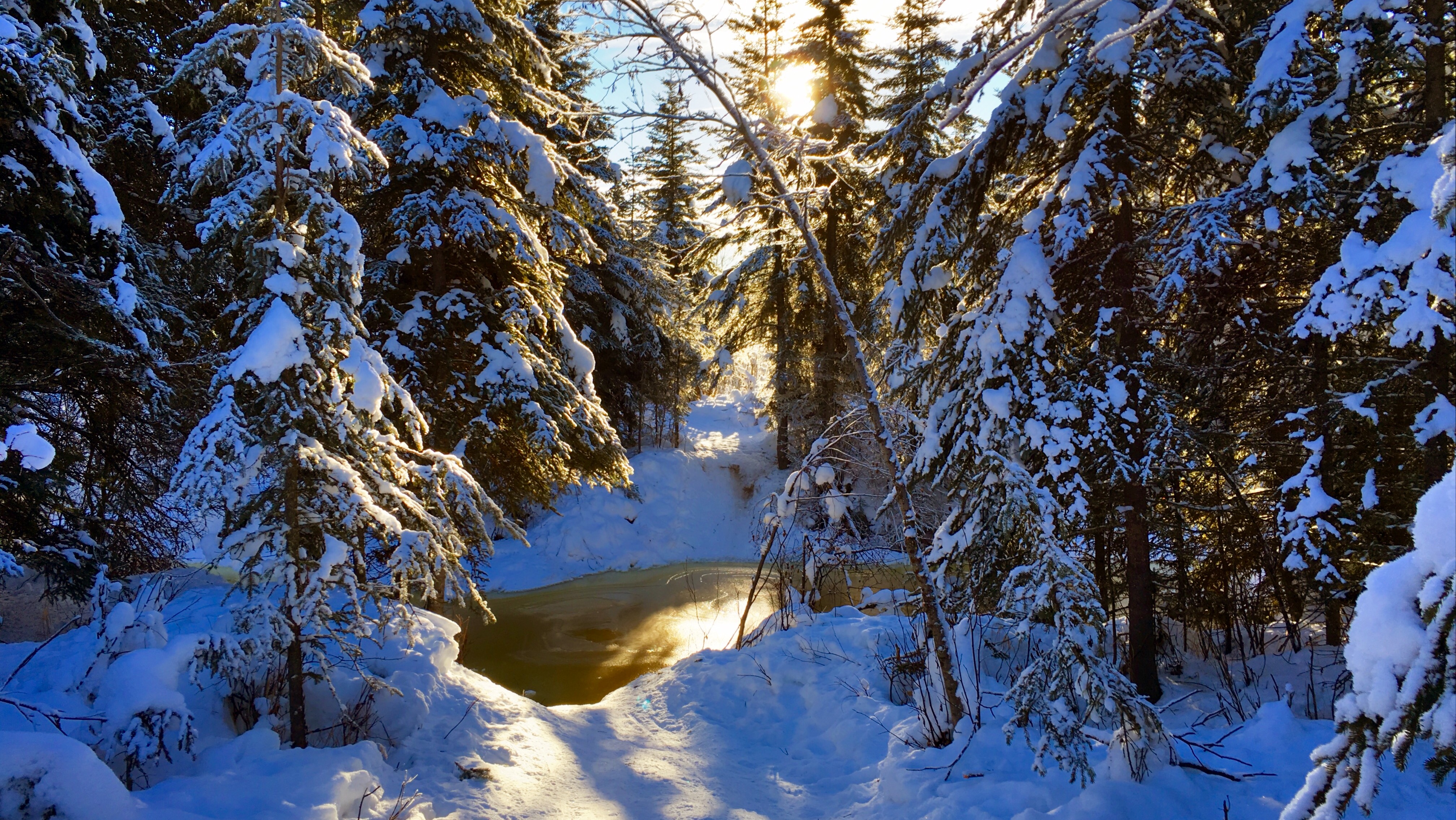
Trail crossing at the end of Miller Hill
Yesterday one of my neighbors sent email with the subject line, “Are we doomed?,” so I took a look at the heigh data from past years. The plot below shows the height of the Creek, as measured from the surface of the bridge (click on the plot to view or download a PDF, R code used to generate the plot appears at the bottom of this post).
The orange region is the region where the Creek is flowing; between my reporting of 0% ice in spring and 100% ice-covered in fall. The data gap in July 2014 was due to the flood washing the bridge downstream. Because the bridge isn’t in the same location, the height measurements before and after the flood aren’t completely comparable, but I don’t have the data for the difference in elevation between the old and new bridge locations, so this is the best we’ve got.

Creek heights by year
The light blue line across all the plots shows the current height of the Creek (3.17 feet) for all years of data. 2012 is probably the closest year to our current situation where the Creek rose to around five feet below the bridge in early January. But really nothing is completely comparable to the situation we’re in right now. Breakup won’t come for another two or three months, and in most years, the Creek rises several feet between February and breakup.
Time will tell, of course, but here’s why I’m not too worried about it. There’s another bridge crossing several miles downstream, and last Friday there was no water on the surface, and the Creek was easily ten feet below the banks. That means that there is a lot of space within the banks of the Creek downstream that can absorb the melting water as breakup happens. I also think that there is a lot of liquid water trapped beneath the ice on the surface in our neighborhood and that water is likely to slowly drain out downstream, leaving a lot of empty space below the surface ice that can accommodate further overflow as the winter progresses. In past years of walking on the Creek I’ve come across huge areas where the top layer of ice dropped as much as six feet when the water underneath drained away. I’m hoping that this happens here, with a lot of the subsurface water draining downstream.
The Creek is always reminding us of how little we really understand what’s going on and how even a small amount of flowing water can become a huge force when that water accumulates more rapidly than the Creek can handle it. Never a dull moment!
Code
library(readr)
library(dplyr)
library(tidyr)
library(lubridate)
library(ggplot2)
library(scales)

wxcoder <- read_csv("data/wxcoder.csv", na=c("-9999"))
feb_2016_incomplete <- read_csv("data/2016_02_incomplete.csv",
                                na=c("-9999"))

wxcoder <- rbind(wxcoder, feb_2016_incomplete)

wxcoder <- wxcoder %>%
   transmute(dte=as.Date(ymd(DATE)), tmin_f=TN, tmax_f=TX, tobs_f=TA,
             tavg_f=(tmin_f+tmax_f)/2.0,
             prcp_in=ifelse(PP=='T', 0.005, as.numeric(PP)),
             snow_in=ifelse(SF=='T', 0.05, as.numeric(SF)),
             snwd_in=SD, below_bridge_ft=HG,
             ice_cover_pct=IC)

creek <- wxcoder %>% filter(dte>as.Date(ymd("2010-05-27")))

creek_w_year <- creek %>%
   mutate(year=year(dte),
         doy=yday(dte))

ice_free_date <- creek_w_year %>%
   group_by(year) %>%
   filter(ice_cover_pct==0) %>%
   summarize(ice_free_dte=min(dte), ice_free_doy=min(doy))

ice_covered_date <- creek_w_year %>%
   group_by(year) %>%
   filter(ice_cover_pct==100, doy>182) %>%
   summarize(ice_covered_dte=min(dte), ice_covered_doy=min(doy))

flowing_creek_dates <- ice_free_date %>%
   inner_join(ice_covered_date, by="year") %>%
   mutate(ymin=Inf, ymax=-Inf)

latest_obs <- creek_w_year %>%
   mutate(rank=rank(desc(dte))) %>%
   filter(rank==1)

current_height_df <- data.frame(
      year=c(2011, 2012, 2013, 2014, 2015, 2016),
      below_bridge_ft=latest_obs$below_bridge_ft)

q <- ggplot(data=creek_w_year %>% filter(year>2010),
            aes(x=doy, y=below_bridge_ft)) +
   theme_bw() +
   geom_rect(data=flowing_creek_dates %>% filter(year>2010),
             aes(xmin=ice_free_doy, xmax=ice_covered_doy, ymin=ymin, ymax=ymax),
             fill="darkorange", alpha=0.4,
             inherit.aes=FALSE) +
   # geom_point(size=0.5) +
   geom_line() +
   geom_hline(data=current_height_df,
              aes(yintercept=below_bridge_ft),
              colour="darkcyan", alpha=0.4) +
   scale_x_continuous(name="",
                      breaks=c(1,32,60,91,
                               121,152,182,213,
                               244,274,305,335,
                               365),
                      labels=c("Jan", "Feb", "Mar", "Apr",
                               "May", "Jun", "Jul", "Aug",
                               "Sep", "Oct", "Nov", "Dec",
                               "Jan")) +
   scale_y_reverse(name="Creek height, feet below bridge",
                   breaks=pretty_breaks(n=5)) +
   facet_wrap(~ year, ncol=1)

width <- 16
height <- 16
rescale <- 0.75
pdf("creek_heights_2010-2016_by_year.pdf",
    width=width*rescale, height=height*rescale)
print(q)
dev.off()
svg("creek_heights_2010-2016_by_year.svg",
    width=width*rescale, height=height*rescale)
print(q)
dev.off()