Abstract
The following is a document-style version of a presentation I gave at work a couple weeks ago. It's a little less useful for a general audience because you don't have access to the same database I have, but I figured it might be useful for someone who is looking at using dplyr or in manipulating the GHCND data from NCDC.
Introduction
Today we’re going to briefly take a look at the GHCND climate database and a couple new R packages (dplyr and tidyr) that make data import and manipulation a lot easier than using the standard library.
For further reading, consult the vignettes for dplyr and tidyr, and download the cheat sheet:
GHCND database
The GHCND database contains daily observation data from locations around the world. The README linked above describes the data set and the way the data is formatted. I have written scripts that process the station data and the yearly download files and insert it into a PostgreSQL database (noaa).
The script for inserting a yearly file (downloaded from http://www1.ncdc.noaa.gov/pub/data/ghcn/daily/by_year/) is here: ghcn-daily-by_year_process.py
“Tidy” data
Without going into too much detail on the subject (read Hadley Wickham’s paper) for more information, but the basic idea is that it is much easier to analyze data when it is in a particular, “tidy”, form. A Tidy dataset has a single table for each type of real world object or type of data, and each table has one column per variable measured and one row per observation.
For example, here’s a tidy table representing daily weather observations with station × date as rows and the various variables as columns.
| Station | Date | tmin_c | tmax_c | prcp | snow | ... |
|---|---|---|---|---|---|---|
| PAFA | 2014-01-01 | 12 | 24 | 0.00 | 0.0 | ... |
| PAFA | 2014-01-01 | 8 | 11 | 0.02 | 0.2 | ... |
| ... | ... | ... | ... | ... | ... | ... |
Getting raw data into this format is what we’ll look at today.
R libraries & data import
First, let’s load the libraries we’ll need:
library(dplyr)      # data import
library(tidyr)      # column / row manipulation
library(knitr)      # tabular export
library(ggplot2)    # plotting
library(scales)     # “pretty” scaling
library(lubridate)  # date / time manipulations
dplyr and tidyr are the data import and manipulation libraries we will use, knitr is used to produce tabular data in report-quality forms, ggplot2 and scales are plotting libraries, and lubridate is a library that makes date and time manipulation easier.
Also note the warnings about how several R functions have been “masked” when we imported dplyr. This just means we'll be getting the dplyr versions instead of those we might be used to. In cases where we need both, you can preface the function with it's package: base::filter would us the normal filter function instead of the one from dplyr.
Next, connect to the database and the three tables we will need:
noaa_db <- src_postgres(host="mason",
                        dbname="noaa")
ghcnd_obs <- tbl(noaa_db, "ghcnd_obs")
ghcnd_vars <- tbl(noaa_db, "ghcnd_variables")
The first statement connects us to the database and the next two create table links to the observation table and the variables table.
Here’s what those two tables look like:
glimpse(ghcnd_obs)
## Observations: 29404870
## Variables:
## $ station_id  (chr) "USW00027502", "USW00027502", "USW00027502", "USW0...
## $ dte         (date) 2011-05-01, 2011-05-01, 2011-05-01, 2011-05-01, 2...
## $ variable    (chr) "AWND", "FMTM", "PRCP", "SNOW", "SNWD", "TMAX", "T...
## $ raw_value   (dbl) 32, 631, 0, 0, 229, -100, -156, 90, 90, 54, 67, 1,...
## $ meas_flag   (chr) "", "", "T", "T", "", "", "", "", "", "", "", "", ...
## $ qual_flag   (chr) "", "", "", "", "", "", "", "", "", "", "", "", ""...
## $ source_flag (chr) "X", "X", "X", "X", "X", "X", "X", "X", "X", "X", ...
## $ time_of_obs (int) NA, NA, 0, NA, NA, 0, 0, NA, NA, NA, NA, NA, NA, N...
glimpse(ghcnd_vars)
## Observations: 82
## Variables:
## $ variable       (chr) "AWND", "EVAP", "MDEV", "MDPR", "MNPN", "MXPN",...
## $ description    (chr) "Average daily wind speed (tenths of meters per...
## $ raw_multiplier (dbl) 0.1, 0.1, 0.1, 0.1, 0.1, 0.1, 0.1, 0.1, 0.1, 0....
Each row in the observation table rows contain the station_id, date, a variable code, the raw value for that variable, and a series of flags indicating data quality, source, and special measurements such as the “trace” value used for precipitation under the minimum measurable value.
Each row in the variables table contains a variable code, description and the multiplier used to convert the raw value from the observation table into an actual value.
This is an example of completely “normalized” data, and it’s stored this way because not all weather stations record all possible variables, and rather than having a single row for each station × date with a whole bunch of empty columns for those variables not measured, each row contains the station × data × variable data.
We are also missing information about the stations, so let’s load that data:
fai_stations <-
    tbl(noaa_db, "ghcnd_stations") %>%
    filter(station_name %in% c("FAIRBANKS INTL AP",
                               "UNIVERSITY EXP STN",
                               "COLLEGE OBSY"))
glimpse(fai_stations)
## Observations: 3
## Variables:
## $ station_id   (chr) "USC00502107", "USW00026411", "USC00509641"
## $ station_name (chr) "COLLEGE OBSY", "FAIRBANKS INTL AP", "UNIVERSITY ...
## $ latitude     (dbl) 64.86030, 64.80389, 64.85690
## $ longitude    (dbl) -147.8484, -147.8761, -147.8610
## $ elevation    (dbl) 181.9656, 131.6736, 144.7800
## $ coverage     (dbl) 0.96, 1.00, 0.98
## $ start_date   (date) 1948-05-16, 1904-09-04, 1904-09-01
## $ end_date     (date) 2015-04-03, 2015-04-02, 2015-03-13
## $ variables    (chr) "TMIN TOBS WT11 SNWD SNOW WT04 WT14 TMAX WT05 DAP...
## $ the_geom     (chr) "0101000020E6100000A5BDC117267B62C0EC2FBB270F3750...
The first part is the same as before, loading the ghcnd_stations table, but we are filtering that data down to just the Fairbanks area stations with long term records. To do this, we use the pipe operator %>% which takes the data from the left side and passes it to the function on the right side, the filter function in this case.
filter requires one or more conditional statements with variable names on the left side and the condition on the right. Multiple conditions can be separated by commas if you want all the conditions to be required (AND) or separated by a logic operator (& for AND, | for OR). For example: filter(latitude > 70, longitude < -140).
When used on database tables, filter can also use conditionals that are built into the database which are passed directly as part of a WHERE clause. In our code above, we’re using the %in% operator here to select the stations from a list.
Now we have the station_ids we need to get just the data we want from the observation table and combine it with the other tables.
Combining data
Here’s how we do it:
fai_raw <-
    ghcnd_obs %>%
    inner_join(fai_stations, by="station_id") %>%
    inner_join(ghcnd_vars, by="variable") %>%
    mutate(value=raw_value*raw_multiplier) %>%
    filter(qual_flag=='') %>%
    select(station_name, dte, variable, value) %>%
    collect()
glimpse(fai_raw)
In order, here’s what we’re doing:
- Assign the result to fai_raw
- Join the observation table with the filtered station data, using station_id as the variable to combine against. Because this is an “inner” join, we only get results where station_id matches in both the observation and the filtered station data. At this point we only have observation data from our long-term Fairbanks stations.
- Join the variable table with the Fairbanks area observation data, using variable to link the tables.
- Add a new variable called value which is calculated by multiplying raw_value (coming from the observation table) by raw_multiplier (coming from the variable table).
- Remove rows where the quality flag is not an empty space.
- Select only the station name, date, variable and actual value columns from the data. Before we did this, each row would contain every column from all three tables, and most of that information is not necessary.
- Finally, we “collect” the results. dplyr doesn’t actually perform the full SQL until it absolutely has to. Instead it’s retrieving a small subset so that we can test our operations quickly. When we are happy with the results, we use collect() to grab the full data.
De-normalize it
The data is still in a format that makes it difficult to analyze, with each row in the result containing a single station × date × variable observation. A tidy version of this data requires each variable be a column in the table, each row being a single date at each station.
To “pivot” the data, we use the spread function, and we'll also calculate a new variable and reduce the number of columns in the result.
fai_pivot <-
    fai_raw %>%
    spread(variable, value) %>%
    mutate(TAVG=(TMIN+TMAX)/2.0) %>%
    select(station_name, dte, TAVG, TMIN, TMAX, TOBS, PRCP, SNOW, SNWD,
           WSF1, WDF1, WSF2, WDF2, WSF5, WDF5, WSFG, WDFG, TSUN)
head(fai_pivot)
## Source: local data frame [6 x 18]
##
##   station_name        dte  TAVG TMIN TMAX TOBS PRCP SNOW SNWD WSF1 WDF1
## 1 COLLEGE OBSY 1948-05-16 11.70  5.6 17.8 16.1   NA   NA   NA   NA   NA
## 2 COLLEGE OBSY 1948-05-17 15.55 12.2 18.9 17.8   NA   NA   NA   NA   NA
## 3 COLLEGE OBSY 1948-05-18 14.40  9.4 19.4 16.1   NA   NA   NA   NA   NA
## 4 COLLEGE OBSY 1948-05-19 14.15  9.4 18.9 12.2   NA   NA   NA   NA   NA
## 5 COLLEGE OBSY 1948-05-20 10.25  6.1 14.4 14.4   NA   NA   NA   NA   NA
## 6 COLLEGE OBSY 1948-05-21  9.75  1.7 17.8 17.8   NA   NA   NA   NA   NA
## Variables not shown: WSF2 (dbl), WDF2 (dbl), WSF5 (dbl), WDF5 (dbl), WSFG
##   (dbl), WDFG (dbl), TSUN (dbl)
spread takes two parameters, the variable we want to spread across the columns, and the variable we want to use as the data value for each row × column intersection.
Examples
Now that we've got the data in a format we can work with, let's look at a few examples.
Find the coldest temperatures by winter year
First, let’s find the coldest winter temperatures from each station, by winter year. “Winter year” is just a way of grouping winters into a single value. Instead of the 2014–2015 winter, it’s the 2014 winter year. We get this by subtracting 92 days (the days in January, February, March) from the date, then pulling off the year.
Here’s the code.
fai_winter_year_minimum <-
    fai_pivot %>%
        mutate(winter_year=year(dte - days(92))) %>%
        filter(winter_year < 2014) %>%
        group_by(station_name, winter_year) %>%
        select(station_name, winter_year, TMIN) %>%
        summarize(tmin=min(TMIN*9/5+32, na.rm=TRUE), n=n()) %>%
        filter(n>350) %>%
        select(station_name, winter_year, tmin) %>%
        spread(station_name, tmin)

last_twenty <-
    fai_winter_year_minimum %>%
        filter(winter_year > 1993)

last_twenty
## Source: local data frame [20 x 4]
##
##    winter_year COLLEGE OBSY FAIRBANKS INTL AP UNIVERSITY EXP STN
## 1         1994       -43.96            -47.92             -47.92
## 2         1995       -45.04            -45.04             -47.92
## 3         1996       -50.98            -50.98             -54.04
## 4         1997       -43.96            -47.92             -47.92
## 5         1998       -52.06            -54.94             -54.04
## 6         1999       -50.08            -52.96             -50.98
## 7         2000       -27.94            -36.04             -27.04
## 8         2001       -40.00            -43.06             -36.04
## 9         2002       -34.96            -38.92             -34.06
## 10        2003       -45.94            -45.94                 NA
## 11        2004           NA            -47.02             -49.00
## 12        2005       -47.92            -50.98             -49.00
## 13        2006           NA            -43.96             -41.98
## 14        2007       -38.92            -47.92             -45.94
## 15        2008       -47.02            -47.02             -49.00
## 16        2009       -32.98            -41.08             -41.08
## 17        2010       -36.94            -43.96             -38.02
## 18        2011       -47.92            -50.98             -52.06
## 19        2012       -43.96            -47.92             -45.04
## 20        2013       -36.94            -40.90                 NA
See if you can follow the code above. The pipe operator makes is easy to see each operation performed along the way.
There are a couple new functions here, group_by and summarize. group_by indicates at what level we want to group the data, and summarize uses those groupings to perform summary calculations using aggregate functions. We group by station and winter year, then we use the minimum and n functions to get the minimum temperature and number of days in each year where temperature data was available. You can see we are using n to remove winter years where more than two weeks of data are missing.
Also notice that we’re using spread again in order to make a single column for each station containing the minimum temperature data.
Here’s how we can write out the table data as a restructuredText document, which can be converted into many document formats (PDF, ODF, HTML, etc.):
sink("last_twenty.rst")
print(kable(last_twenty, format="rst"))
sink()
| winter_year | COLLEGE OBSY | FAIRBANKS INTL AP | UNIVERSITY EXP STN |
|---|---|---|---|
| 1994 | -43.96 | -47.92 | -47.92 |
| 1995 | -45.04 | -45.04 | -47.92 |
| 1996 | -50.98 | -50.98 | -54.04 |
| 1997 | -43.96 | -47.92 | -47.92 |
| 1998 | -52.06 | -54.94 | -54.04 |
| 1999 | -50.08 | -52.96 | -50.98 |
| 2000 | -27.94 | -36.04 | -27.04 |
| 2001 | -40.00 | -43.06 | -36.04 |
| 2002 | -34.96 | -38.92 | -34.06 |
| 2003 | -45.94 | -45.94 | NA |
| 2004 | NA | -47.02 | -49.00 |
| 2005 | -47.92 | -50.98 | -49.00 |
| 2006 | NA | -43.96 | -41.98 |
| 2007 | -38.92 | -47.92 | -45.94 |
| 2008 | -47.02 | -47.02 | -49.00 |
| 2009 | -32.98 | -41.08 | -41.08 |
| 2010 | -36.94 | -43.96 | -38.02 |
| 2011 | -47.92 | -50.98 | -52.06 |
| 2012 | -43.96 | -47.92 | -45.04 |
| 2013 | -36.94 | -40.90 | NA |
Plotting
Finally, let’s plot the minimum temperatures for all three stations.
q <-
    fai_winter_year_minimum %>%
        gather(station_name, tmin, -winter_year) %>%
        arrange(winter_year) %>%
        ggplot(aes(x=winter_year, y=tmin, colour=station_name)) +
            geom_point(size=1.5, position=position_jitter(w=0.5,h=0.0)) +
            geom_smooth(method="lm", se=FALSE) +
            scale_x_continuous(name="Winter Year", breaks=pretty_breaks(n=20)) +
            scale_y_continuous(name="Minimum temperature (degrees F)", breaks=pretty_breaks(n=10)) +
            scale_color_manual(name="Station",
                               labels=c("College Observatory",
                                        "Fairbanks Airport",
                                        "University Exp. Station"),
                               values=c("darkorange", "blue", "darkcyan")) +
            theme_bw() +
            # theme(legend.position = c(0.150, 0.850)) +
            theme(axis.text.x = element_text(angle=45, hjust=1))

print(q)
To plot the data, we need the data in a slightly different format with each row containing winter year, station name and the minimum temperature. We’re plotting minimum temperature against winter year, coloring the points and trendlines using the station name. That means all three of those variables need to be on the same row.
To do that we use gather. The first parameter is the name of variable the columns will be moved into (the station names, which are currently columns, will become values in a row named station_name). The second is the name of the column that stores the observations (tmin) and the parameters after that are the list of columns to gather together. In our case, rather than specifying the names of the columns, we're specifying the inverse: all the columns except winter_year.
The result of the gather looks like this:
fai_winter_year_minimum %>%
    gather(station_name, tmin, -winter_year)
## Source: local data frame [321 x 3]
##
##    winter_year station_name tmin
## 1         1905 COLLEGE OBSY   NA
## 2         1907 COLLEGE OBSY   NA
## 3         1908 COLLEGE OBSY   NA
## 4         1909 COLLEGE OBSY   NA
## 5         1910 COLLEGE OBSY   NA
## 6         1911 COLLEGE OBSY   NA
## 7         1912 COLLEGE OBSY   NA
## 8         1913 COLLEGE OBSY   NA
## 9         1915 COLLEGE OBSY   NA
## 10        1916 COLLEGE OBSY   NA
## ..         ...          ...  ...
ggplot2
The plot is produced using ggplot2. A full introduction would be a seminar by itself, but the basics of our plot can be summarized as follows.
ggplot(aes(x=winter_year, y=tmin, colour=station_name)) +
aes defines variables and grouping.
geom_point(size=1.5, position=position_jitter(w=0.5,h=0.0)) +
geom_smooth(method="lm", se=FALSE) +
geom_point draws points, geom_smooth draws fitted lines.
scale_x_continuous(name="Winter Year", breaks=pretty_breaks(n=20)) +
scale_y_continuous(name="Minimum temperature (degrees F)",
                    breaks=pretty_breaks(n=10)) +
scale_color_manual(name="Station",
                    labels=c("College Observatory", "Fairbanks Airport",
                            "University Exp. Station"),
                    values=c("darkorange", "blue", "darkcyan")) +
Scale functions define how the data is scaled into a plot and controls labelling.
theme_bw() +
theme(axis.text.x = element_text(angle=45, hjust=1))
Theme functions controls the style.
For more information:
Linear regression, winter year and minimum temperature
Finally let’s look at the significance of those regression lines:
summary(lm(data=fai_winter_year_minimum, `COLLEGE OBSY` ~ winter_year))
##
## Call:
## lm(formula = `COLLEGE OBSY` ~ winter_year, data = fai_winter_year_minimum)
##
## Residuals:
##      Min       1Q   Median       3Q      Max
## -19.0748  -5.8204   0.1907   3.8042  17.1599
##
## Coefficients:
##               Estimate Std. Error t value Pr(>|t|)
## (Intercept) -275.01062  105.20884  -2.614   0.0114 *
## winter_year    0.11635    0.05311   2.191   0.0325 *
## ---
## Signif. codes:  0 '***' 0.001 '**' 0.01 '*' 0.05 '.' 0.1 ' ' 1
##
## Residual standard error: 7.599 on 58 degrees of freedom
##   (47 observations deleted due to missingness)
## Multiple R-squared:  0.07643,    Adjusted R-squared:  0.06051
## F-statistic:   4.8 on 1 and 58 DF,  p-value: 0.03249
summary(lm(data=fai_winter_year_minimum, `FAIRBANKS INTL AP` ~ winter_year))
##
## Call:
## lm(formula = `FAIRBANKS INTL AP` ~ winter_year, data = fai_winter_year_minimum)
##
## Residuals:
##     Min      1Q  Median      3Q     Max
## -15.529  -4.605  -1.025   4.007  19.764
##
## Coefficients:
##               Estimate Std. Error t value Pr(>|t|)
## (Intercept) -171.19553   43.55177  -3.931 0.000153 ***
## winter_year    0.06250    0.02221   2.813 0.005861 **
## ---
## Signif. codes:  0 '***' 0.001 '**' 0.01 '*' 0.05 '.' 0.1 ' ' 1
##
## Residual standard error: 7.037 on 104 degrees of freedom
##   (1 observation deleted due to missingness)
## Multiple R-squared:  0.07073,    Adjusted R-squared:  0.06179
## F-statistic: 7.916 on 1 and 104 DF,  p-value: 0.005861
summary(lm(data=fai_winter_year_minimum, `UNIVERSITY EXP STN` ~ winter_year))
##
## Call:
## lm(formula = `UNIVERSITY EXP STN` ~ winter_year, data = fai_winter_year_minimum)
##
## Residuals:
##     Min      1Q  Median      3Q     Max
## -15.579  -5.818  -1.283   6.029  19.977
##
## Coefficients:
##               Estimate Std. Error t value Pr(>|t|)
## (Intercept) -158.41837   51.03809  -3.104  0.00248 **
## winter_year    0.05638    0.02605   2.164  0.03283 *
## ---
## Signif. codes:  0 '***' 0.001 '**' 0.01 '*' 0.05 '.' 0.1 ' ' 1
##
## Residual standard error: 8.119 on 100 degrees of freedom
##   (5 observations deleted due to missingness)
## Multiple R-squared:  0.04474,    Adjusted R-squared:  0.03519
## F-statistic: 4.684 on 1 and 100 DF,  p-value: 0.03283
Essentially, all the models show a significant increase in minimum temperature over time, but none of them explain very much of the variation in minimum temperature.
RMarkdown
This presentation was produced with the RMarkdown package. Allows you to mix text and R code, which is then run through R to produce documents in Word, PDF, HTML, and presentation formats.
Last night we got a quarter of an inch of rain at our house, making roads “impassable” according to the Fairbanks Police Department, and turning the dog yard, deck, and driveway into an icy mess. There are videos floating around Facebook showing Fairbanks residents playing hockey in the street in front of their houses, and a reported seven vehicles off the road on Ballaine Hill.
Here’s a video of a group of Goldstream Valley musicians ice skating on Golstream Road: http://youtu.be/_afC7UF0NXk
Let’s check out the weather database and take a look at how often Fairbanks experiences this type of event, and when they usually happen. I’m going to skip the parts of the code showing how we get pivoted daily data from the database, but they’re in this post.
Starting with pivoted data we want to look for dates from November through March with more than a tenth of an inch of precipitation, snowfall less than two tenths of an inch and a daily high temperature above 20°F. Then we group by the winter year and month, and aggregate the rain events into a single event. These occurrences are rare enough that this aggregation shoudln’t combine events from different parts of the month.
Here’s the R code:
winter_rain <-
   fai_pivot %>%
      mutate(winter_year=year(dte - days(92)),
               wdoy=yday(dte + days(61)),
               month=month(dte),
               SNOW=ifelse(is.na(SNOW), 0, SNOW),
               TMAX=TMAX*9/5+32,
               TAVG=TAVG*9/5+32,
               TMIN=TMIN*9/5+32,
               PRCP=PRCP/25.4,
               SNOW=SNOW/25.4) %>%
      filter(station_name == 'FAIRBANKS INTL AP',
               winter_year < 2014,
               month %in% c(11, 12, 1, 2, 3),
               TMAX > 20,
               PRCP > 0.1,
               SNOW < 0.2) %>%
      group_by(winter_year, month) %>%
      summarize(date=min(dte), tmax=mean(TMAX),
                prcp=sum(PRCP), days=n()) %>%
      ungroup() %>%
      mutate(month=month(date)) %>%
      select(date, month, tmax, prcp, days) %>%
      arrange(date)
And the results:
| Date | Month | Max temp (°F) | Rain (inches) | Days |
|---|---|---|---|---|
| 1921-03-07 | 3 | 44.06 | 0.338 | 1 |
| 1923-02-06 | 2 | 33.98 | 0.252 | 1 |
| 1926-01-12 | 1 | 35.96 | 0.142 | 1 |
| 1928-03-02 | 3 | 39.02 | 0.110 | 1 |
| 1931-01-19 | 1 | 33.08 | 0.130 | 1 |
| 1933-11-03 | 11 | 41.00 | 0.110 | 1 |
| 1935-11-02 | 11 | 38.30 | 0.752 | 3 |
| 1936-11-24 | 11 | 37.04 | 0.441 | 1 |
| 1937-01-10 | 1 | 32.96 | 1.362 | 3 |
| 1948-11-10 | 11 | 48.02 | 0.181 | 1 |
| 1963-01-19 | 1 | 35.06 | 0.441 | 1 |
| 1965-03-29 | 3 | 35.96 | 0.118 | 1 |
| 1979-11-11 | 11 | 35.96 | 0.201 | 1 |
| 2003-02-08 | 2 | 34.97 | 0.291 | 2 |
| 2003-11-02 | 11 | 34.97 | 0.268 | 2 |
| 2010-11-22 | 11 | 34.34 | 0.949 | 3 |
This year’s event doesn’t compare to 2010 when almost and inch of rain fell over the course of three days in November, but it does look like it comes at an unusual part of the year.
Here’s the counts and frequency of winter rainfall events by month:
by_month <-
   winter_rain %>%
      group_by(month) %>%
      summarize(n=n()) %>%
      mutate(freq=n/sum(n)*100)
| Month | n | Freq |
|---|---|---|
| 1 | 4 | 25.00 |
| 2 | 2 | 12.50 |
| 3 | 3 | 18.75 |
| 11 | 7 | 43.75 |
There haven’t been any rain events in December, which is a little surprising, but next to that, February rains are the least common.
I looked at this two years ago (Winter freezing rain) using slightly different criteria. At the bottom of that post I looked at the frequency of rain events over time and concluded that they seem to come in cycles, but that the three events in this decade was a bad sign. Now we can add another rain event to the total for the 2010s.
Over the past couple days in Fairbanks, there has been a strong flow of warm, moist air from the Pacific which culminated in a record (for January 14th) 0.22 inches of precipitation, most of which fell as rain. Nasty. Similar events happened in 2011 and in November 2010, which everyone will remember for the inch or more of ice that glazed the roads for the rest of the winter that year.
The question people always ask after a series of events like this is whether this is a new weather pattern (let’s hope not!) and whether it may be the result of global climate change (which I probably can’t answer).
To look at this, I examined the historical record for Fairbanks, searching for dates that met the following criteria:
- At least six inches of snow on the ground
- During the winter months (October through February)
- Daily high temperature above freezing
- Precipitation falling as rain
The last criteria isn’t part of the historical record, but we can guess the amount of rain by comparing the amount of snow (measured each day on a snow board that is cleared after measurement) with the amount of liquid precipitation gathered in a tube and melted, if necessary. In my experience, the ratio of snow to liquid precipitation is almost always less than 10 to 1 (meaning that 10 inches of snow melts down to less than an inch of liquid), so I’m looking for dates where the precipitation amount is greater than 10 times the snowfall for that date. I’m also estimating the amount of rain by subtracting (snow × 10) from the precipitation total.
Here’s the query:
SELECT dte, tmin_f, tmax_f, prcp_in, snow_in, rain_in,
       row_number() OVER (ORDER BY rain_in desc) AS rank
FROM (
    SELECT to_char(dte, 'YYYY-MM') AS dte, round(avg(tmin_f), 1) AS tmin_f,
           round(avg(tmax_f), 1) AS tmax_f, sum(prcp_in) AS prcp_in,
           sum(snow_in) AS snow_in, sum(rain_in) AS rain_in
    FROM (
        SELECT dte, tmin_f, tmax_f, prcp_in, snow_in, snwd_in,
               round(prcp_in - (snow_in / 10.0), 2) AS rain_in
        FROM get_ghcnd('Fairbanks Intl Ap')
        WHERE extract(month from dte) IN (10, 11, 12, 1, 2)
            AND snwd_in > 6
            AND tmax_f > 32
            AND prcp_in * 10 > snow_in
        ORDER BY dte
    ) AS foo
    GROUP BY to_char(dte, 'YYYY-MM')
) AS bar
ORDER BY dte;
And the results, ordered by the year and month of the event. None of the winter rain events stretched across a month boundary, so it was convenient to aggregate them this way (although 1937 is problematic as I mention below).
| Date | Min Temp (°F) | Max Temp (°F) | Precip (in) | Snow (in) | “Rain” (in) | Rank |
|---|---|---|---|---|---|---|
| 1920-02 | 27.7 | 38.4 | 0.26 | 0.9 | 0.17 | 11 |
| 1931-01 | 12.0 | 33.1 | 0.13 | 0.0 | 0.13 | 12 |
| 1932-02 | 7.0 | 33.1 | 0.77 | 7.1 | 0.06 | 16 |
| 1933-11 | 25.0 | 41.0 | 0.11 | 0.0 | 0.11 | 14 |
| 1935-11 | 30.4 | 37.2 | 1.51 | 3.2 | 1.19 | 2 |
| 1936-11 | 30.0 | 37.0 | 0.44 | 0.0 | 0.44 | 5 |
| 1937-01 | 24.3 | 36.2 | 2.83 | 16.1 | 1.22 | 1 |
| 1941-02 | 28.0 | 42.1 | 0.02 | 0.0 | 0.02 | 23 |
| 1941-11 | -2.9 | 33.1 | 0.20 | 0.9 | 0.11 | 15 |
| 1943-02 | 30.5 | 41.0 | 0.12 | 0.0 | 0.12 | 13 |
| 1944-02 | 21.5 | 36.5 | 0.65 | 2.9 | 0.36 | 7 |
| 1948-01 | 7.0 | 33.1 | 0.01 | 0.0 | 0.01 | 26 |
| 1957-01 | 30.9 | 35.1 | 0.03 | 0.0 | 0.03 | 22 |
| 1961-01 | 17.1 | 33.1 | 0.04 | 0.0 | 0.04 | 20 |
| 1963-01 | 22.5 | 35.1 | 0.56 | 0.7 | 0.49 | 4 |
| 1967-12 | 20.0 | 33.1 | 0.43 | 0.5 | 0.38 | 6 |
| 1970-02 | 10.9 | 43.0 | 0.05 | 0.0 | 0.05 | 17 |
| 1970-10 | 28.0 | 44.1 | 0.04 | 0.0 | 0.04 | 19 |
| 1970-12 | 5.0 | 36.0 | 0.43 | 2.4 | 0.19 | 9 |
| 1986-02 | 10.9 | 37.9 | 0.03 | 0.0 | 0.03 | 21 |
| 1989-02 | 24.1 | 37.0 | 0.40 | 3.8 | 0.02 | 24 |
| 2003-02 | 27.0 | 35.0 | 0.29 | 0.0 | 0.29 | 8 |
| 2006-02 | 17.1 | 42.1 | 0.06 | 0.1 | 0.05 | 18 |
| 2010-11 | 26.1 | 34.3 | 0.95 | 0.1 | 0.94 | 3 |
| 2011-12 | 26.1 | 46.9 | 0.03 | 0.2 | 0.01 | 25 |
| 2013-01 | 24.0 | 37.0 | 0.22 | 0.4 | 0.18 | 10 |
The 2010 event was had the third highest rainfall in the historical record; yesterday’s rain was the tenth highest. The January 1937 event is actually two events, one on the 10th and 11th and one on the 20th and 21st. If we split them up into two events, the 2010 rainfall amount is the second largest amount and the two January 1937 rainfalls come in third and tied for fifth, with November 1935 holding the record.
Grouping the events into decades, we get the following:
| Decade | Rain events |
|---|---|
| 1920s | 1 |
| 1930s | 6 |
| 1940s | 5 |
| 1950s | 1 |
| 1960s | 3 |
| 1970s | 3 |
| 1980s | 2 |
| 1990s | 0 |
| 2000s | 2 |
| 2010s | 3 |
Here’s a visualization of the same data:
I don’t think there’s evidence that what we’ve seen in the last few years is exceptional in the historical record, but it does seem like the frequency of winter rainfall does come in cycles, with a peak in the 30s and 40s, and something of a decline in the 80s and 90s. That we’ve already had three events in this decade, in just over two years, seems like a bad sign to me. I wonder if there are larger scale climatological phenomena that could help to explain the pattern shown here?
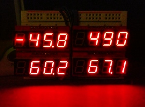
-45.8°F outside
It seems like it’s been cold for almost the entire winter this year, with the exception of the few days last week when we got more than 16 inches of snow. Unfortunately, it’s been hard to enjoy it, with daily high temperatures typically well below -20°F.
Let’s see how this winter ranks among the early-season Fairbanks winters going back to 1904. To get an estimate of how cold the winter is, I’m adding together all the daily average temperatures (in degrees Celsius) for each day from October 1st through yesterday. Lower values for this sum indicate colder winters.
Here’s the SQL query. The CASE WHEN stuff is to include the recent data that isn’t in the database I was querying.
SELECT year,
    CASE WHEN year = 2012 THEN cum_deg - 112 ELSE cum_deg END AS cum_deg,
    rank() OVER (
        ORDER BY CASE WHEN year = 2012 THEN cum_deg - 112 ELSE cum_deg END
    ) AS rank
FROM (
    SELECT year, round(sum(tavg_c) AS cum_deg
    FROM (
        SELECT extract(year from dte) AS year,
            extract(doy from dte) AS doy,
            tavg_c
        FROM ghcnd_obs
        WHERE station_id = 'USW00026411'
        ORDER BY year, doy
    ) AS foo
    WHERE doy between extract(doy from '2011-10-01'::date)
                  and extract(doy from '2012-12-19'::date)
    GROUP BY year ORDER BY year
) AS bar
ORDER by rank;
And the results: this has been the fifth coldest early-season winter since 1904.
| O/N/D rank | year | O/N/D cumulative °C | N/D rank |
|---|---|---|---|
| 1 | 1917 | -1550 | 1 |
| 2 | 1956 | -1545 | 4 |
| 3 | 1977 | -1451 | 3 |
| 4 | 1975 | -1444 | 5 |
| 5 | 2012 | -1388 | 7 |
| 6 | 1946 | -1380 | 2 |
| 7 | 1999 | -1337 | 12 |
| 8 | 1966 | -1305 | 9 |
| 9 | 1942 | -1303 | 6 |
| 10 | 1935 | -1298 | 10 |
In addition to the ranks for October through today (O/N/D rank in the table), the last column (N/D rank) shows the same calculation without October temperatures. It’s always a good idea to examine how well a relationship holds up when the interval is manipulated in order to see if the results are an artifact of the choice of period. In this case, the rankings change, but not dramatically.
Tonight we may cross -50°F for the first time this year at our house, but even without the very cold temperatures predicted (but not record cold) through the weekend, the start of the 2012/2013 winter has been exceptionally chilly.
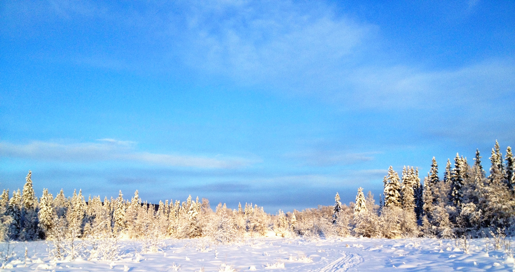
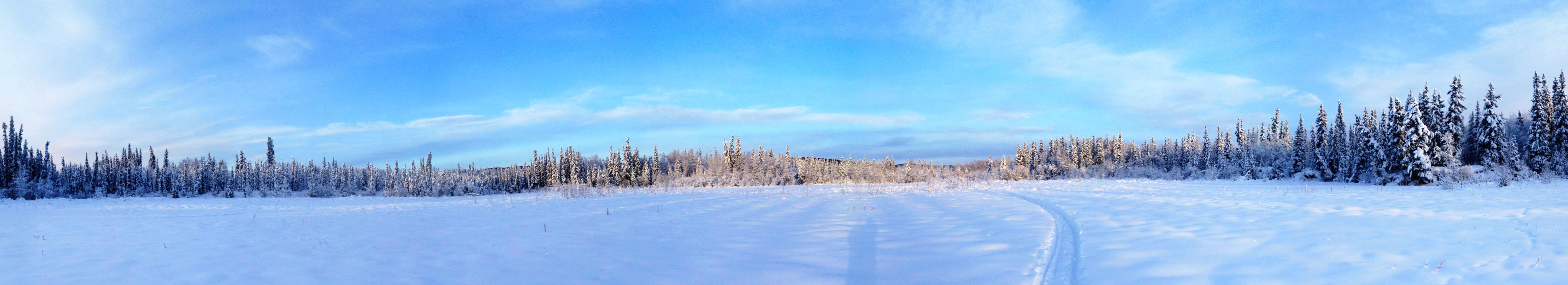
Frozen pond on Goldstream Creek
It was -25°F at the house, but the sun was out and I couldn’t resist going for a ski. Goldstream Creek has been going through an extended period of overflowing for most of the winter, so I wasn’t sure how far I would get. I skied on the Valley trail toward Ballaine Road, turned down the hill at the DNR pond, and skied west (sort of!) on the Creek until it met up with the power line trail. I took that trail east until connecting to the trail up the hill to Shadow Lane. Then down Shadow to the edge of our Miller Hill property and back down to the Valley trail. It was 3.5 miles, and polar wax was just about right. The sun, snow and trail conditions made it a great ski. I’m sure the two people skijouring with their dogs and the musher I crossed paths with will agree.
Here’s a panorama taken from a location close to the photo to the right (click on either for a larger version).