I re-ran the analysis of my ski speeds discussed in an earlier post. The model looks like this:
lm(formula = mph ~ season_days + temp, data = ski)

Residuals:
     Min       1Q   Median       3Q      Max
-1.76466 -0.20838  0.02245  0.15600  0.90117

Coefficients:
            Estimate Std. Error t value Pr(>|t|)
(Intercept) 4.414677   0.199258  22.156  < 2e-16 ***
season_days 0.008510   0.001723   4.938 5.66e-06 ***
temp        0.027334   0.003571   7.655 1.10e-10 ***
---
Signif. codes:  0 ‘***’ 0.001 ‘**’ 0.01 ‘*’ 0.05 ‘.’ 0.1 ‘ ’ 1

Residual standard error: 0.428 on 66 degrees of freedom
Multiple R-squared: 0.5321, Adjusted R-squared: 0.5179
F-statistic: 37.52 on 2 and 66 DF,  p-value: 1.307e-11
What this is saying is that about half the variation in my ski speeds can be explained by the temperature when I start skiing and how far along in the season we are (season_days). Temperature certainly makes sense—I was reminded of how little glide you get at cold temperatures skiing to work this week at -25°F. And it’s gratifying that my speeds are increasing as the season goes on. It’s not my imagination that my legs are getting stronger and my technique better.
The following figure shows the relationship of each of these two variables (season_days and temp) to the average speed of the trip. I used the melt function from the reshape package to make the plot:
melted <- melt(data = ski,
               measure.vars = c('season_days', 'temp'),
               id.vars = 'mph')
q <- ggplot(data = melted, aes(x = value, y = mph))
q + geom_point()
  + facet_wrap(~ variable, scales = 'free_x')
  + stat_smooth(method = 'lm')
  + theme_bw()
Last week I replaced by eighteen-year-old ski boots with a new pair, and they’re hurting my ankles a little. Worse, the first four trips with my new boots were so slow and frustrating that I thought maybe I’d made a mistake in the pair I’d bought. My trip home on Friday afternoon was another frustrating ski until I stopped and applied warmer kick wax and had a much more enjoyable mile and a half home. There are a lot of other unmeasured factors including the sort of snow on the ground (fresh snow vs. smooth trail vs. a trail ripped up by snowmachines), whether I applied the proper kick wax or not, whether my boots are hurting me, how many times I stopped to let dog teams by, and many other things I can’t think of. Explaining half of the variation in speed is pretty impressive.
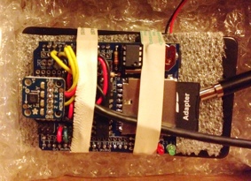
Today was the first day where I got some good data skiing to and from work using my data logger. There’s a photo of it in it’s protective box on the right. The Arduino and data logging shield (with the sensors soldered to it) is sitting on top of a battery pack holding six AA batteries. The accelerometer is the little square board that is sticking up on the left side of the logger, and you can see the SD card on the right side. The cord under the rubber bands leads to the external temperature sensor.
This morning it took about four minutes for the sensor to go from room temperature to outside temperature (-12°F), which means I need to pre-acclimate it before going out for a ski. A thermocouple would respond faster (much less mass), but they’re not as accurate because they have such a wide response range (-200°C to 1,350°C). A thermistor might be a good compromise, but I haven’t fiddled with those yet.
Here’s the temperature data from my ski home:
When I left work, the temperature at our house was 12°F, and I figured it would be warmer almost everywhere else, so I used “extra green” kick wax, which has a range of 12 to 21°F. I’ve highlighted this range on the plot with a transparent green box. In general, if you’ve chosen wax that’s too warm for the conditions, you won’t get much glide, and if the wax is rated too cold, you won’t have much kick. The plot shows that as I got near the end of the route and the temperature dropped below the lower range of the wax, I should have lost some glide, which is pretty much exactly what happened. Normally this isn’t a big issue on the Goldstream Valley Trail because it’s often very smooth, which means that a warmer wax is needed to get a grip, but this afternoon’s trail had seen a lot of snowmachine traffic, it wasn’t very smooth, and I didn’t get as much glide as earlier in the ski.
The other interesting thing is the dramatic dip marked “Goldstream Creek” on the plot. This is where the trail crosses the Creek on a small bridge designed for light recreational traffic (nothing bigger than a snowmachine or four-wheeler). It’s probably the lowest place in the trail. Our house is also on the Creek, so the two coldest spots on the trail are exactly where I’d expect them to be, right on the Creek.

Skiing at -34
This morning I skied to work at the coldest temperatures I’ve ever attempted (-31°F when I left). We also got more than an inch of snow yesterday, so not only was it cold, but I was skiing in fresh snow. It was the slowest 4.1 miles I’d ever skied to work (57+ minutes!) and as I was going, I thought about what factors might explain how fast I ski to and from work.
Time to fire up R and run some PostgreSQL queries. The first query grabs the skiing data for this winter:
SELECT start_time,
    (extract(epoch from start_time) - extract(epoch from '2011-10-01':date))
        / (24 * 60 * 60) AS season_days,
    mph,
    dense_rank() OVER (
        PARTITION BY
            extract(year from start_time)
            || '-' || extract(week from start_time)
        ORDER BY date(start_time)
    ) AS week_count,
    CASE WHEN extract(hour from start_time) < 12 THEN 'morning'
         ELSE 'afternoon'
    END AS time_of_day
FROM track_stats
WHERE type = 'Skiing'
    AND start_time > '2011-07-03' AND miles > 3.9;
This yields data that looks like this:
| start_time | season_days | miles | mph | week_count | time_of_day |
|---|---|---|---|---|---|
| 2011-11-30 06:04:21 | 60.29469 | 4.11 | 4.70 | 1 | morning |
| 2011-11-30 15:15:43 | 60.67758 | 4.16 | 4.65 | 1 | afternoon |
| 2011-12-02 06:01:05 | 62.29242 | 4.07 | 4.75 | 2 | morning |
| 2011-12-02 15:19:59 | 62.68054 | 4.11 | 4.62 | 2 | afternoon |
Most of these are what you’d expect. The unconventional ones are season_days, the number of days (and fraction of a day) since October 1st 2011; week_count, the count of the number of days in that week that I skied. What I really wanted week_count to be was the number of days in a row I’d skied, but I couldn’t come up with a quick SQL query to get that, and I think this one is pretty close.
I got this into R using the following code:
library(lubridate)
library(ggplot2)
library(RPostgreSQL)
drv <- dbDriver("PostgreSQL")
con <- dbConnect(drv, dbname=...)
ski <- dbGetQuery(con, query)
ski$start_time <- ymd_hms(as.character(ski$start_time))
ski$time_of_day <- factor(ski$time_of_day, levels = c('morning', 'afternoon'))
Next, I wanted to add the temperature at the start time, so I wrote a function in R that grabs this for any date passed in:
get_temp <- function(dt) {
    query <- paste("SELECT ... FROM arduino WHERE obs_dt > '",
        dt,
        "' ORDER BY obs_dt LIMIT 1;", sep = "")
    temp <- dbGetQuery(con, query)
    temp[[1]]
}
The query is simplified, but the basic idea is to build a query that finds the next temperature observation after I started skiing. To add this to the existing data:
temps <- sapply(ski[,'start_time'], FUN = get_temp)
ski$temp <- temps
Now to do some statistics:
model <- lm(data = ski, mph ~ season_days + week_count + time_of_day + temp)
Here’s what I would expect. I’d think that season_days would be positively related to speed because I should be getting faster as I build up strength and improve my skill level. week_count should be negatively related to speed because the more I ski during the week, the more tired I will be. I’m not sure if time_of_day is relevant, but I always get the sense that I’m faster on the way home so afternoon should be positively associated with speed. Finally, temp should be positively associated with speed because the glide you can get from a properly waxed pair of skis decreases as the temperature drops.
Here's the results:
summary(model)
Coefficients:
                     Estimate  Std. Error t value Pr(>|t|)
(Intercept)          4.143760   0.549018   7.548 1.66e-08 ***
season_days          0.006687   0.006097   1.097  0.28119
week_count           0.201717   0.087426   2.307  0.02788 *
time_of_dayafternoon 0.137982   0.143660   0.960  0.34425
temp                 0.021539   0.007694   2.799  0.00873 **
---
Signif. codes:  0 ‘***’ 0.001 ‘**’ 0.01 ‘*’ 0.05 ‘.’ 0.1 ‘ ’ 1

Residual standard error: 0.4302 on 31 degrees of freedom
Multiple R-squared: 0.4393,    Adjusted R-squared: 0.367
F-statistic: 6.072 on 4 and 31 DF,  p-value: 0.000995
The model is significant, and explains about 37% of the variation in speed. The only variables that are significant are week_count and temp, but oddly, week_count is positively associated with speed, meaning the more I ski during the week, the faster I get by the end of the week. That doesn’t make any sense, but it may be because the variable isn’t a good proxy for the “consecutive days” variable I was hoping for. Temperature is positively associated with speed, which means that I ski faster when it’s warmer.
The other refinement to this model that might have a big impact would be to add a variable for how much snow fell the night before I skied. I am fairly certain that the reason this morning’s -31°F ski was much slower than my return home at -34°F was because I was skiing on an inch of fresh snow in the morning and had tracks to ski in on the way home.
Frozen pond on Goldstream Creek
It was -25°F at the house, but the sun was out and I couldn’t resist going for a ski. Goldstream Creek has been going through an extended period of overflowing for most of the winter, so I wasn’t sure how far I would get. I skied on the Valley trail toward Ballaine Road, turned down the hill at the DNR pond, and skied west (sort of!) on the Creek until it met up with the power line trail. I took that trail east until connecting to the trail up the hill to Shadow Lane. Then down Shadow to the edge of our Miller Hill property and back down to the Valley trail. It was 3.5 miles, and polar wax was just about right. The sun, snow and trail conditions made it a great ski. I’m sure the two people skijouring with their dogs and the musher I crossed paths with will agree.
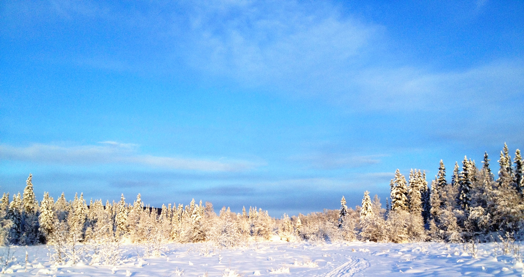
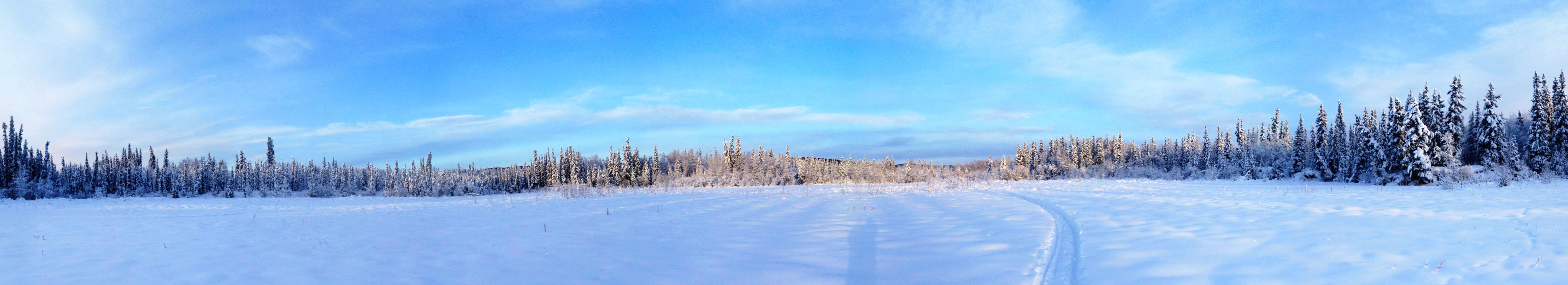
Here’s a panorama taken from a location close to the photo to the right (click on either for a larger version).

Skiing home
This year I’ve made a serious effort to improve my physical fitness. I started lifting weights in August, and worked hard to commute to work as much as I could by bicycle (6.7 miles each way) or ski (4.1 miles). I commuted on 102 days this year, which is 40% of the possible work days in the year. I also spent a lot of time out on the trails with our now 15-year old dog, Nika. In May, I set up a standing desk at work, and as I’ll demonstrate below, this is a significant improvement over spending all those hours sitting, at least for energy consumption. As a result of all this, I feel like I am in the best shape of my life, and that makes me feel good as I enter middle age.
Here’s the summary of what I did this year (details on the calculations appear below):
| Activity | Miles | Hours | Speed | Energy |
|---|---|---|---|---|
| Treadmill | 8.98 | 1.58 | 5.62 | 925 |
| Skiing | 268.35 | 54.25 | 4.98 | 27,685 |
| Bicycling | 960.22 | 69.67 | 13.86 | 38,606 |
| Hiking | 201.06 | 81.56 | 2.53 | 28,750 |
| Skating | 3.49 | 0.75 | 4.65 | 236 |
| Lifting | 56.10 | 19,775 | ||
| TOTAL | 1,442 | 263.91 | 115,976 |
The other thing I did was start standing up at my desk at work. I spent 1,258 hours at my desk after I started standing. According to the Compendium of Physical Activities, standing at work consumes 2.3 metabolic equivalent units (MET). This is the ratio of work metabolic rate over resting metabolic rate, which would be 1.0 MET. Thus, standing uses an additional 1.3 MET over resting. Sitting at a desk is 1.5 MET, which means standing adds 0.8 MET.
To use these numbers, you need an estimate of your resting metabolic rate. Using the Mifflin et al. equation on this page I get 1,691 Kcal/day, or 70.5 Kcal per hour for my height, weight, and age. For those 1,258 hours standing at work I burned an additional 71 thousand calories: 1,258 • 0.8 • 70.5 = 70,951 Kcal (the “calories” reported on food labels are technically kilocalories (Kcal) in energy units). That’s a lot of energy, just by standing instead of sitting.
The energy values in the table above were also calculated using the same methods. I fiddled with the tabular values from the compendium and got the following approximations:
- Running MET = 1.653 • speed (mph)
- Skiing = ((speed - 2.5) / 2) + 7
- Bicycling = speed - 5
- Hiking = 6
- Skating = 5.5
- Lifting = 6
Despite the amount of energy consumed by standing instead of sitting at work, I think there is a real benefit to the more intense exercises listed in the table. These strengthen and build skeletal and cardiovascular muscle in ways that simply standing all day don’t.
When all the numbers are totaled, I burned an extra 512 calories (318 exercising, 194 standing) each day in 2011. That’s certainly worth a beer or two, and I look and feel better for it even drinking them!